
pgvector vs a Dedicated Vector Database: Memory, Filters, and Index Builds


TL;DR pgvector is the right default for embeddings that belong to Postgres rows, until one of three limits shows up in measurements: the HNSW index outgrows the memory it gets, filtered queries lose recall or latency, or index builds start competing with the workload. A dedicated vector database like Qdrant handled filtered search far better in my tests. Under the same memory cap it fell off the same cliff until it was configured for quantization, and it adds a second system to keep in sync.
An embedding is a list of numbers, 768 of them in this post, that a model produces for a piece of text. Semantic search means finding the stored embeddings closest to the one for a query, and doing that exactly means comparing the query against every row. Both systems here avoid that with an approximate index called HNSW: a graph that links each vector to a handful of its near neighbors, which a query walks from an entry point toward its target while keeping a short list of the best candidates found so far. The length of that list is the search-effort setting, hnsw.ef_search in pgvector and hnsw_ef in Qdrant. A longer list finds more of the true nearest rows and takes longer. The share it finds is recall, so a recall of 0.958 means about nine and a half of the true ten came back.
The choice is where that index lives. pgvector is a Postgres extension that adds a vector column type and HNSW indexes, so the embeddings sit in the same table as the rows they describe and a search is an ORDER BY in SQL. A dedicated vector database (Qdrant, Pinecone, Milvus, Weaviate) is a separate service built for this one kind of search. Choosing it buys an engine tuned for the job, and costs a second system that has to receive a copy of every embedding and every filter value. This post loads the same 500,000 embeddings into pgvector and into Qdrant and runs both through the same tests.
Here are the results first, and how they were measured after. Latencies are medians, and the last two rows are reasoned rather than measured.
| Question | pgvector | Qdrant | Edge |
|---|---|---|---|
| Plain top-10 at similar recall | 0.958 at 2.82 ms | 0.940 at 2.31 ms | Close |
| Filter on a few known values | 0.960 at 0.71 ms, partial index | 1.0 at 2.52 ms | pgvector on speed, Qdrant on recall |
| Filter nobody can enumerate | 0.867 at 19.6 ms | 1.0 at 2.52 ms | Qdrant |
| Index outgrows memory, default config | 209 ms | 1,296 ms | pgvector |
| Index outgrows memory, compressed | 73.7 ms at 0.906 | 4.26 ms at 0.935 | Qdrant, by far less at p99 |
| Rebuild on a live table | 196 s, writes keep landing | 79 to 388 s in the background, behavior during it untested | Unsettled |
| Deleted row leaves search results | At commit | When the sync pipeline catches up | pgvector |
| Restore to one point in time | One restore | Two restores or a full re-sync | pgvector |
Here is one nearest-neighbor query run twice against the same 1,953 MB HNSW index, on PostgreSQL 18.6 with pgvector 0.8.7. The plan is identical and both runs touch 1,198 buffers. Output is trimmed to the lines that differ.
 1
 2
 3
 4
 5
 6
 7
 8
 9
10
11
12
-- index fits in shared_buffers (2,560 MB)
Limit (actual time=1.853..1.898 rows=10.00 loops=1)
 Buffers: shared hit=1198
 -> Index Scan using items_hnsw on items (actual time=1.852..1.898 rows=10.00 loops=1)
Execution Time: 1.903 ms

-- container capped at 1 GB, shared_buffers 256 MB, disk capped at 3,000 read IOPS
Limit (actual time=296.405..297.841 rows=10.00 loops=1)
 Buffers: shared hit=356 read=842
 I/O Timings: shared read=294.552
 -> Index Scan using items_hnsw on items (actual time=296.402..297.833 rows=10.00 loops=1)
Execution Time: 297.885 ms
Nothing about the query changed. In the second run 842 of the pages the graph walk needed were not in memory, and each one cost a read from a disk throttled to the gp3 baseline. Waiting for those reads took 294 of the 298 milliseconds. The earlier post on the hidden costs of an AI rollout covers storage growth, halfvec, and buffer-cache pollution on a shared OLTP box, so none of that is repeated here.
The fixture is 500,000 real embeddings: 768-dimensional InstructorXL vectors of arXiv paper titles, the first ten parquet files of Qdrant’s public arxiv-titles-instructorxl-embeddings dataset. The arXiv identifier encodes the submission year, which gives a real metadata column to filter on. Research topics shift over the decades, so it is correlated with the vectors rather than random. The 1,000 query vectors come from an eleventh file, so none of them is in the table, and recall@10 is scored against an exact search over the same 500,000 rows in numpy. Both systems got HNSW with m = 16 and ef_construction = 64 on cosine distance, with 4 CPUs and a 3.5 GB memory limit in Docker. Latency is measured at the client, one connection, 1,000 queries after a 200-query warm-up on different vectors. Qdrant is 1.20.0, queried over gRPC.
What half a million vectors can show This ran on a laptop whose Docker VM has 5 CPUs and 4.9 GB of RAM, which is what capped the fixture at 500,000 vectors. Each limit below shows up at this scale, but the absolute numbers belong to this box, and nothing here exercises what a billion vectors brings (sharding, rebuilds measured in days).
On unfiltered queries the two systems are close.
| Search effort | pgvector recall | pgvector p50 / p99 | Qdrant recall | Qdrant p50 / p99 |
|---|---|---|---|---|
| 40 | 0.908 | 2.18 / 3.65 ms | 0.940 | 2.31 / 3.40 ms |
| 100 | 0.958 | 2.82 / 4.33 ms | 0.982 | 3.07 / 4.22 ms |
| 200 | 0.977 | 4.91 / 7.11 ms | 0.993 | 4.94 / 6.83 ms |
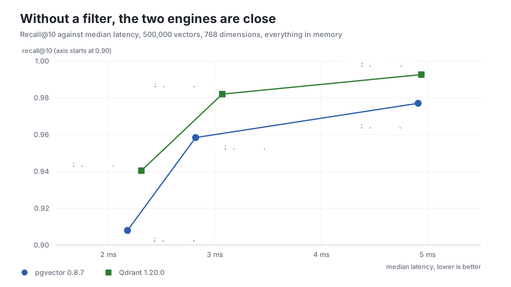
The same search-effort number is not the same amount of work in the two systems. Qdrant split the collection into three segments with a graph each and searches all three, so its 40 explores more candidates than pgvector’s 40. That is why the first row reads 0.940 against 0.908. Compared at matched recall instead, a dedicated engine buys a millisecond or two of median latency on plain top-10 search.
Filtered search is where the gap opens
pgvector applies a WHERE clause after the index scan, not during it. The README says so directly: with the default hnsw.ef_search of 40 and a condition that matches 10% of rows, “only 4 rows will match on average.” The scan produces at most 40 candidates, the filter throws most of them away, and the LIMIT 10 is satisfied by whatever survives.
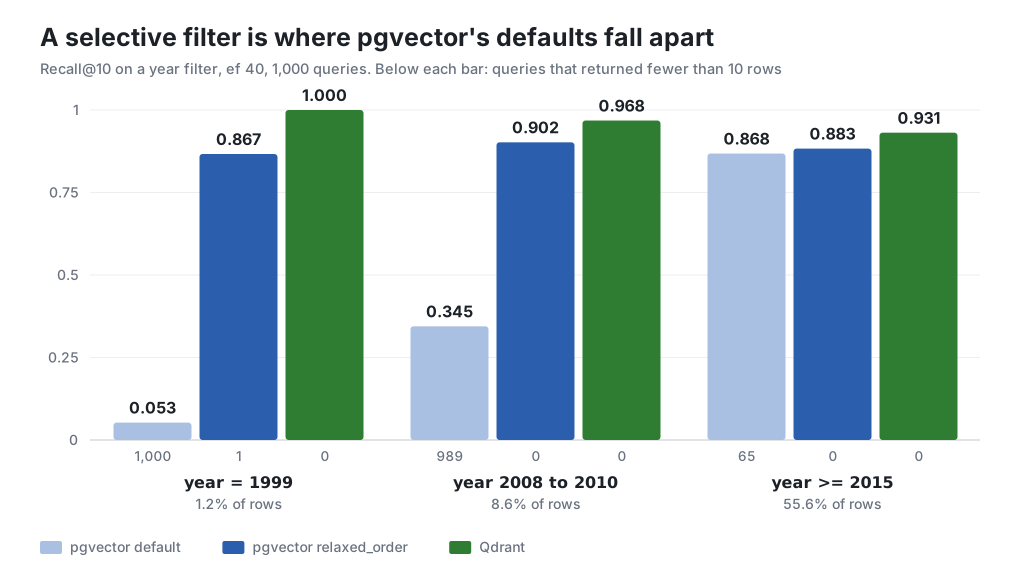
On this fixture year = 1999 matches 5,863 rows (1.2%). With pgvector’s defaults, recall@10 was 0.053 and every one of the 1,000 queries returned fewer than ten rows. Nothing errors and nothing warns. Alex Jacobs’ The Case Against pgvector (October 2025, 381 points on Hacker News) described this as asking for ten results and getting three; the tables below show what that looks like across a thousand queries.
The obvious repair is a B-tree on year. I added one and ran ANALYZE, expecting the planner to use it for a 1.2% filter, and it kept the HNSW plan and the 0.053 recall. Raising ef_search flipped it (60 was already enough, with iterative scans still off). The planner switched to a Bitmap Heap Scan on the B-tree plus a sort, which is an exact search: recall 1.0 at 18.0 ms. That flip comes from the cost-estimation change in pgvector 0.8.0 (November 2024), and it means the plan choice is made by a cost estimate in which recall plays no part. At ef_search = 40 the cheapest-looking plan was the one that returned 5% of the right answer.
Defaults return short results without an error With hnsw.iterative_scan off, which is the default, a filtered pgvector query can return fewer rows than its LIMIT and nothing in the result says so. Turn on iterative scans for filtered queries, and count rows against the limit in the application, because a short result is the only visible symptom.
Iterative scans, also new in 0.8.0, keep walking the graph until enough rows pass the filter or hnsw.max_scan_tuples (default 20,000) is reached. Here is everything I tried on the 1.2% filter:
Strategy for year = 1999 | Recall@10 | p50 | p99 | Queries short of 10 rows |
|---|---|---|---|---|
| pgvector defaults | 0.053 | 2.88 ms | 7.05 ms | 1,000 |
| B-tree, plan flipped to exact search | 1.0 | 18.0 ms | 21.2 ms | 0 |
strict_order iterative scan | 0.795 | 22.3 ms | 36.4 ms | 1 |
relaxed_order iterative scan | 0.867 | 19.6 ms | 36.3 ms | 1 |
| Partial HNSW index | 0.960 | 0.71 ms | 0.91 ms | 0 |
| Qdrant with a payload index | 1.0 | 2.52 ms | 3.75 ms | 0 |
strict_order ran before the B-tree existed; relaxed_order with and without it came in within 2 ms of each other. Raising max_scan_tuples to 100,000 moved recall by a thousandth, so on this filter the graph itself sets the ceiling. Across selectivities, the gap closes as the filter loosens:
| Filter (rows matched) | pgvector default | pgvector relaxed_order | Exact via B-tree | Qdrant 1.20 |
|---|---|---|---|---|
year = 1999 (1.2%) | 0.053, 2.9 ms | 0.867, 19.6 ms | 1.0, 18.0 ms | 1.0, 2.52 ms |
2008–2010 (8.6%) | 0.345, 2.0 ms | 0.902, 4.1 ms | 1.0, 97 ms | 0.968, 2.18 ms |
year >= 2015 (55.6%) | 0.868, 2.1 ms | 0.883, 1.6 ms | not run | 0.931, 2.42 ms |
Each cell is recall@10 and median latency, with search effort at 40. The medians hide the tail: relaxed_order reached a 36 ms p99 on the 1.2% filter and 28 ms on the 8.6% one, while Qdrant stayed under 4 ms on all three. At an effort of 100 on the 55.6% filter, pgvector reached 0.945 at 2.74 ms and Qdrant 0.981 at 3.16 ms.
Partial indexes are the README’s answer when a filter has a few known values, and the partial-index row shows they work, built in under a second at 23 MB. The catch is one index per value. That covers a status flag or a handful of large tenants, and it stops covering anything once filters are combinations (tenant and date range and document permission) that nobody can enumerate ahead of time.
Qdrant handled all three filters at roughly unfiltered latency because it plans per segment with the filter’s cardinality in hand. Its query planner uses the payload index to estimate how many points match, scans small sets directly, and searches the graph with filter-aware extra edges when the set is large. The indexing docs also say the extra edges only exist when the payload index is created before the HNSW graph, so adding a new filter field later means rebuilding.
The memory cliff is not a pgvector problem
The opening plans are the endpoints of a ladder: one pgvector index, one query, less memory at each step.
| Setup | p50 | p95 | p99 |
|---|---|---|---|
Index in shared_buffers, 3.5 GB container | 2.18 ms | 3.02 ms | 3.65 ms |
shared_buffers 256 MB, index in OS page cache | 3.42 ms | 4.56 ms | 5.31 ms |
| Container capped at 1 GB | 6.01 ms | 8.06 ms | 9.45 ms |
| 1 GB and 3,000 read IOPS | 209 ms | 395 ms | 400 ms |
| Control: 3.5 GB, 3,000 read IOPS, index resident | 2.02 ms | 3.64 ms | 44.3 ms |
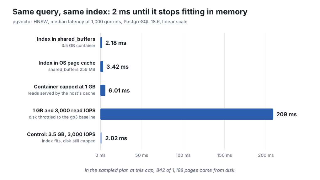
The third row looked far too good, and I believed it for one full run before the per-query plans showed why: 687 to 925 page reads at 10 to 15 microseconds each. Docker Desktop’s VM disk is a file on the Mac, and the Mac’s own page cache was serving those “disk” reads from RAM. To give a read a real cost, I capped the volume at 3,000 read IOPS through the container’s cgroup, which is the gp3 baseline. The control row isolates the cap: with the index resident the median did not move, though the p99 went from 3.65 ms to 44 ms.
Qdrant with its default configuration, full-precision vectors held in memory, hit the same wall harder, at about six times pgvector’s median under the same constraint. I did not dig into why. The claim that a dedicated engine has no memory cliff did not survive this test. It has one wherever its working set stops fitting.
| Under 1 GB and 3,000 read IOPS | p50 | p95 | p99 | Recall@10 | p50 with memory to spare |
|---|---|---|---|---|---|
| Qdrant, default config | 1,296 ms | 1,608 ms | 1,800 ms | 0.946 | 2.31 ms |
| pgvector HNSW | 209 ms | 395 ms | 400 ms | 0.906 | 2.18 ms |
| pgvector binary index, 200-candidate rerank | 73.7 ms | 97.5 ms | 106 ms | 0.906 | 4.42 ms |
| Qdrant int8, rescoring on | 4.26 ms | 67.9 ms | 79.3 ms | 0.935 | not run |
| Qdrant int8, no rescoring | 0.74 ms | 1.27 ms | 1.64 ms | 0.915 | 0.63 ms |
The Qdrant default row is 300 queries instead of 1,000, because each one took over a second, and that smaller sample is why its recall reads 0.946 rather than 0.940. pgvector’s 0.906 against the earlier 0.908 comes from the index being rebuilt between runs.
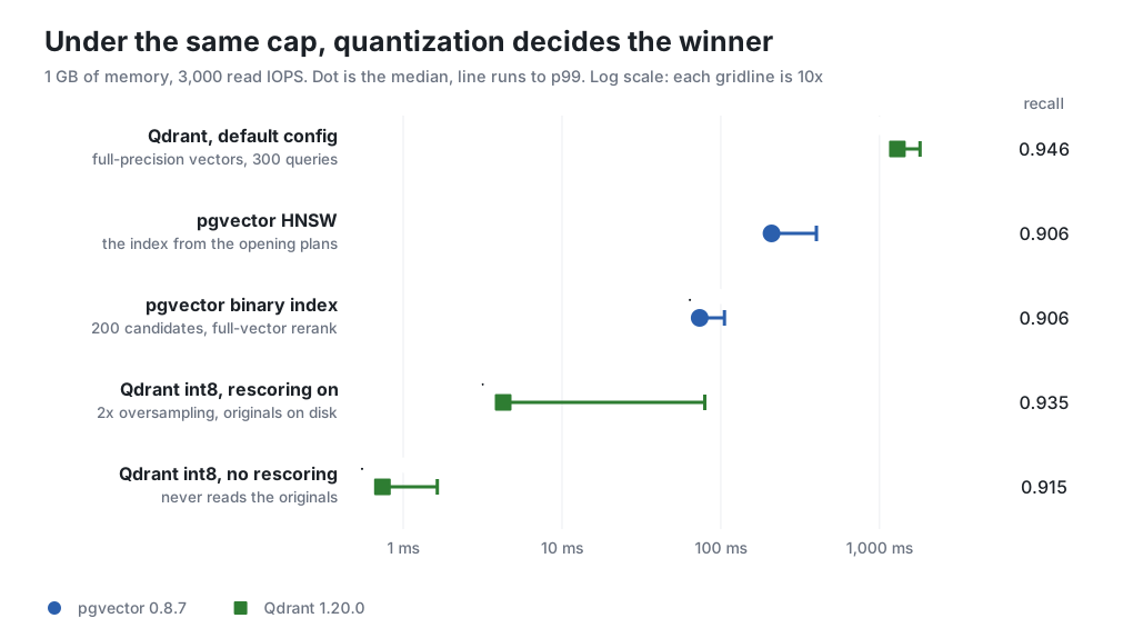
Where the dedicated engine pulls ahead is the configuration that avoids the cliff. A second Qdrant collection with scalar quantization keeps int8 copies in RAM and the originals on disk. Qdrant does not rescore 8-bit quantization by default, so the last row never read the originals. Rescoring with 2x oversampling bought back recall and cost a 79 ms p99, because those reads now hit the throttled disk. pgvector has no int8 vector type. Its nearest tool is a binary-quantized expression index with a full-precision rerank in SQL. Binary codes lose more than int8 on this model (0.703 recall from 40 candidates, 0.838 from 100), so it took 200 candidates to reach 0.906. Under the cap, each of those candidates is a full vector fetched from TOAST on the throttled disk.
So both systems get past the cliff the same way, by keeping a compressed copy in memory and touching the full vectors as little as possible. On this fixture Qdrant did it about 17 times faster at the median for slightly better recall. The tail is far closer, 79 ms against 106 ms at p99, because both end up waiting on the same throttled disk. Qdrant offers the technique as two collection settings. pgvector makes it a query pattern and an extra index you maintain, built on a coarser code. The dedicated engine has one more advantage that no benchmark here captures: it is the only tenant of its memory, while pgvector’s index shares shared_buffers with every other query on the primary.
That sharing is also the build-time problem. My first attempt at the build test ran with shared_buffers at 2,560 MB so the index would stay resident, and the OOM killer took it out twice. A parallel HNSW build with maintenance_work_mem = 2GB and a buffer pool sized to hold the finished index do not both fit in 3.5 GB.
Index builds block only if you let them
A plain CREATE INDEX on the 500,000 rows took 167.3 s with three parallel workers and produced the 1,953 MB index. Then I ran both forms with a writer inserting one row every 100 ms:
| Build with a live writer | Build time | Inserts landed | Insert p50 | Insert p99 | Longest insert |
|---|---|---|---|---|---|
CREATE INDEX | 175.6 s | 82 | 9.11 ms | 33.4 s | 175.5 s |
CREATE INDEX CONCURRENTLY | 196.2 s | 1,808 | 3.26 ms | 72.5 ms | 723 ms |
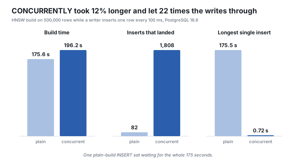
This is the measurement that pushes back hardest on the thesis. Blocking is opt-out, the README says to build concurrently in production, and a team that reads it will never see the 175-second stall. What stays true at scale is duration. The build is a full pass over every vector on the primary, and its time grows with the corpus. An embedding-model change forces it again on a corpus that has kept growing since the last time. A concurrent build that fails partway leaves an INVALID index behind that has to be dropped or reindexed before it is any use. That is ordinary Postgres behavior, and it hurts more when a retry costs hours.
Qdrant moves the build off the write path. The upload with indexing deferred took about 24 s (the Postgres COPY of the same rows took 84 s), and the optimizer then built the graphs in the background:
| What got built | Time | Size on disk |
|---|---|---|
| pgvector HNSW | 167.3 s | 1,953 MB |
| pgvector binary expression index | 37.3 s | 190 MB |
pgvector partial index, year = 1999 | 0.89 s | 23 MB |
| Qdrant graphs, no payload index | 152 s after upload | not measured |
Qdrant graphs with payload index on year | 388 s after upload | 1.7 GB, whole collection |
Qdrant int8 collection, payload index on year | 78.7 s after upload | 2.8 GB, whole collection |
Postgres holds every vector twice, 2,000 MB in the table (all but 25 MB of it TOAST) and again inside the index. So the HNSW row sits on top of the table, while Qdrant’s 1.7 GB is the whole collection. Compression was not free on disk either: the int8 collection came to 2.8 GB. It also built fastest of the three Qdrant collections while carrying the same payload index, so the gap between 152 s and 388 s is not simply the price of filter-aware edges. I did not chase why. Each upload finished before its graph build started, so I measured neither writes nor query latency during a Qdrant build. Points in segments that have not been indexed yet are searched without the graph. How searches behave during a rebuild is untested here.
What the second system costs
Everything above argues for the dedicated engine on filtered search and for treating memory as a configuration question on both sides. The bill for it sits in the parts this benchmark did not touch.
Sync comes first. The embeddings are derived from rows that live in Postgres, so every insert, update, and delete has to reach the vector store. A dual write from the application is not atomic. A crash between the Postgres commit and the Qdrant upsert leaves the stores disagreeing, and nothing notices until a search returns a row that no longer exists. The designs that hold up are an outbox table or logical decoding feeding a consumer, and both add a pipeline with its own lag and its own place to page someone.
Deletes are the sharp end. In pgvector a revoked permission or a deleted document leaves search results when the transaction commits. In a second store it stays searchable, and quotable by whatever model sits downstream, for as long as the pipeline is behind.
Filters have to be copied. The year column here went into Qdrant as payload, which was easy because it never changes. Real filters, such as tenant, status, and who can see the document, live in other tables and change on their own schedule. Each change becomes a payload update in the second system, and a new filter field means a new payload index and a graph rebuild. The joins go too. A query that ranks by distance and joins to a permissions table in one statement becomes an ID list from one system and a lookup in the other, the coupling you can’t see until you split.
Backups and restores double, and they do not line up. Qdrant snapshots cover one collection on one node and restore to the same or next minor version, and there is no shared point in time with a Postgres base backup and WAL. A restore of both systems is two restores and a reconciliation, or one restore and a full re-sync from Postgres, which on this fixture is a 24-second upload followed by 388 seconds of indexing. At the scale where the dedicated engine starts to make sense, that re-sync grows with the corpus.
All of this assumes Postgres is on the menu. On MySQL Community 26.10.0 a VECTOR column exists, takes up to 16,383 dimensions, and does very little else. DISTANCE() fails with ERROR 1305, because the manual reserves it for HeatWave on OCI and MySQL AI and leaves it out of both the Community and Commercial distributions. CREATE INDEX fails with Non-scalar (e.g., vector) column 'e' cannot be used as key. So the server stores an embedding it can neither compare nor index, which makes the headline feature a float array with a nicer name. MariaDB, the fork, has had a VECTOR INDEX built on a modified HNSW since 11.7, generally available in the 11.8 LTS. On stock MySQL, vector search means computing distances in the application, moving to HeatWave, or paying for the second system priced above.
The numbers to watch
Three numbers decide this, and all three can be read off a running Postgres before anyone proposes a migration.
The first is the HNSW index size from pg_relation_size against the memory left over after the rest of the working set. Here the gap between fitting and not fitting was 2 ms against 209 ms. EXPLAIN (ANALYZE, BUFFERS) on a sample of vector queries shows the approach early as shared read counts climbing from zero toward the 842 in the opening plan.
The second is how often filtered vector queries return fewer rows than their LIMIT, plus recall measured offline against the same query with enable_indexscan = off. A sustained short-result rate after iterative scans are on, on filters too varied for partial indexes, is the clearest measured case for the dedicated engine.
The third is the CREATE INDEX CONCURRENTLY duration against how often the corpus gets re-embedded. On this box that was 196 seconds for half a million vectors.