How to Read EXPLAIN ANALYZE: PostgreSQL

TL;DR EXPLAIN ANALYZE runs your query and shows each step PostgreSQL took to answer it, how long each step took, and how many rows it expected at each step next to how many it got. The habit this post teaches is to find the one slow step first and read only its numbers before changing anything. The output tells you where the time went, not why, so the fix still takes some thinking.

Plain EXPLAIN shows what PostgreSQL plans to do with your query without running it, so every number in it is a guess. EXPLAIN ANALYZE runs the query for real and prints the same plan with what happened at each step: rows out, time taken, and how much of the table was read. A plan can look sensible and still read the whole table, and only the second command shows that. You can paste the output into an AI and get a reading back, and it will often point at the right line. What it does not know is your system: which table is the busy one, what the query is for, whether a number that looks large is normal here. That judgment is yours, and this post is about having enough of it to check the reading rather than take it.

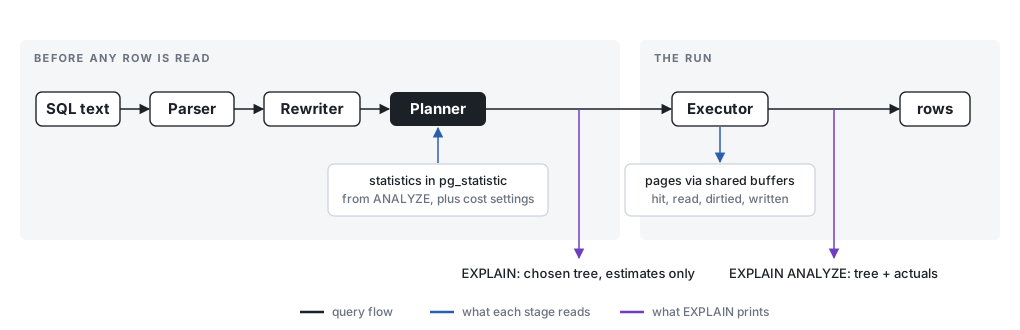
The part of PostgreSQL that decides how to run a query is the planner, and it decides before reading any data. It lists the ways it could answer (read the whole table or use an index, which table to start a join with), estimates the cost of each, and picks the cheapest. Its estimates come from statistics that the ANALYZE command collects, such as how many rows a table has and which values are common. It never looks at the data itself, which is why plain EXPLAIN answers instantly and why it can be wrong.

The executor then runs the chosen plan and counts what happens. EXPLAIN ANALYZE prints those counts next to the planner’s guesses, and reading it mostly means comparing the two.

Every plan below comes from PostgreSQL 18.6 in Docker with default settings, on a customers table of 200,000 rows (50 countries, 10 cities each) and an orders table of 5,000,000. Each order belongs to a random customer, so one customer’s orders are scattered across the table, the way real orders arrive. I turned off JIT compilation and parallel workers to keep the output short. The MySQL version of this post uses the same rows.

What the output is telling you

Start with the simplest slow query there is: one customer’s orders.

1

SELECT id, created_at, total FROM orders WHERE customer_id = 4242;

Plain EXPLAIN prints this:

1
2

 Seq Scan on orders (cost=0.00..145287.00 rows=26 width=22)
 Filter: (customer_id = 4242)

A plan with one step. Seq Scan (sequential scan, or table scan) means read every row of the table from start to finish. Filter is the WHERE condition, checked against each row. rows=26 is the estimate: the planner expects 26 matches. cost is the planner’s price in its own units, not milliseconds. Now with EXPLAIN ANALYZE:

1
2
3
4
5
6

 Seq Scan on orders (cost=0.00..145287.00 rows=26 width=22) (actual time=3.082..144.209 rows=27.00 loops=1)
 Filter: (customer_id = 4242)
 Rows Removed by Filter: 4999973
 Buffers: shared hit=8694 read=74093
 Planning Time: 0.091 ms
 Execution Time: 144.249 ms

The first parenthesis is still the guess. The second is what happened. actual time=3.082..144.209 is milliseconds until the step produced its first row and its last row. rows=27.00 is the rows it produced, so the guess of 26 was close. loops=1 is how many times the step ran, which matters later.

The next two lines are the price. Rows Removed by Filter: 4999973 says PostgreSQL looked at all 5,000,000 rows and threw away all but 27. Buffers counts pages: PostgreSQL stores a table in 8 KB pages of dozens of rows each, and always reads whole pages. shared hit is pages already in its memory cache (shared buffers), and read is pages it asked the operating system for. Together they are 82,787 pages, the whole table. Execution Time is the total, 144 ms.

The estimate was right and the query was still slow, because without an index there was no faster way to find 27 rows than reading everything. An index is a separate sorted structure, like the index at the back of a book, that maps each customer_id to the pages holding that customer’s rows. After CREATE INDEX ON orders (customer_id):

1
2
3
4
5
6
7
8
9

 Bitmap Heap Scan on orders (cost=4.63..107.58 rows=26 width=22) (actual time=0.006..0.014 rows=27.00 loops=1)
 Recheck Cond: (customer_id = 4242)
 Heap Blocks: exact=27
 Buffers: shared hit=30
 -> Bitmap Index Scan on orders_customer_id_idx (cost=0.00..4.63 rows=26 width=0) (actual time=0.003..0.003 rows=27.00 loops=1)
 Index Cond: (customer_id = 4242)
 Index Searches: 1
 Buffers: shared hit=3
 Execution Time: 0.019 ms

Now the plan has two steps, called nodes. A line starting with -> is a node that feeds rows to the node above it, and the deeper it is indented, the earlier it runs. Read innermost first.

The innermost node, Bitmap Index Scan, looked up 4242 in the index (Index Cond), found 27 entries, and read 3 index pages. It hands the row locations up to Bitmap Heap Scan, which fetches those rows from the table (PostgreSQL calls a table’s storage the heap). Heap Blocks: exact=27 says the 27 rows sat on 27 different pages. A parent’s time and buffers include its children’s, so the top Buffers: shared hit=30 is 3 index pages plus 27 table pages. Thirty pages instead of 82,787, and 0.019 ms instead of 144.

EXPLAIN ANALYZE really runs the query For a SELECT it takes as long as the query takes. For UPDATE, DELETE or INSERT the change really happens, so wrap it in BEGIN; and ROLLBACK;, as the PostgreSQL documentation suggests. Run long queries on a copy or a replica, not the server your users are on.

When the database guessed wrong

When the planner guesses wrong it can pick the wrong plan, so the estimate is worth checking on every slow step. This query joins the two tables (a join matches rows in one table to rows in another, here customers to their orders) and totals the orders of every customer in one city:

1
2
3
4

SELECT count(*), sum(o.total)
FROM customers c
JOIN orders o ON o.customer_id = c.id
WHERE c.country = 'C07' AND c.city = 'C07-3';

 1
 2
 3
 4
 5
 6
 7
 8
 9
10
11
12
13
14
15
16
17

 Aggregate (cost=5137.70..5137.71 rows=1 width=40) (actual time=91.548..91.554 rows=1.00 loops=1)
 Buffers: shared hit=3861 read=8553 written=5
 -> Nested Loop (cost=4.63..5136.69 rows=200 width=6) (actual time=0.110..90.336 rows=9940.00 loops=1)
 Buffers: shared hit=3861 read=8553 written=5
 -> Seq Scan on customers c (cost=0.00..4274.00 rows=8 width=4) (actual time=0.010..6.803 rows=400.00 loops=1)
 Filter: ((country = 'C07'::text) AND (city = 'C07-3'::text))
 Rows Removed by Filter: 199600
 Buffers: shared hit=1274
 -> Bitmap Heap Scan on orders o (cost=4.63..107.58 rows=26 width=10) (actual time=0.044..0.205 rows=24.85 loops=400)
 Recheck Cond: (c.id = customer_id)
 Heap Blocks: exact=9940
 Buffers: shared hit=2587 read=8553 written=5
 -> Bitmap Index Scan on orders_customer_id_idx (cost=0.00..4.63 rows=26 width=0) (actual time=0.014..0.014 rows=24.85 loops=400)
 Index Cond: (customer_id = c.id)
 Index Searches: 400
 Buffers: shared hit=785 read=415
 Execution Time: 91.591 ms

Read it inside out. Seq Scan on customers reads all 200,000 customers and keeps the ones in that city. It expected 8 and found 400. That is the thing to look for: estimated rows against actual rows on the same line.

The planner assumes country and city are unrelated, so it multiplies their odds: 200,000 customers, times 1 in 50 for the country, times 1 in 500 for the city, is 8. In this data the city already decides the country, which the planner had no way to know, and the mistake carries up the tree: Nested Loop expected 200 rows and produced 9,940.

Nested Loop is one way to do a join: for each row from its first child (a customer), it runs its second child once (find that customer’s orders through the index). That is what loops=400 on the orders side means. When loops is above 1, rows and actual time are averages per run, so multiply them back: 24.85 rows times 400 is the 9,940, and 0.205 ms times 400 is 82 ms, most of the 91. Buffers are already totals.

Here the wrong guess did no harm, because with 8 customers or 400, looking up each one’s orders in the index is a good plan. A gap like this matters when the right number would have made the planner choose a different plan, and the bigger the gap, the more likely that is. Uniqueness and Selectivity shows one that went from 50 ms to 50 minutes.

Next thing to learn: teaching the planner about related columns CREATE STATISTICS customers_country_city (dependencies) ON country, city FROM customers, then ANALYZE customers, tells PostgreSQL the two columns move together. The estimate went from 8 to 398 and the query got no faster, because the plan did not need to change. Fixing an estimate and fixing a query are different jobs.

When the plan is fine but still slow

The first plan already showed the second lesson: a correct estimate and a slow query, given away by Rows Removed by Filter and Buffers. Here it is in a bigger tree to practice on, a query listing every order since November 1 with its customer’s location, largest total first:

 1
 2
 3
 4
 5
 6
 7
 8
 9
10
11
12
13
14
15
16
17

 Sort (cost=234697.30..236254.94 rows=623058 width=24) (actual time=512.409..573.290 rows=608001.00 loops=1)
 Sort Key: o.total DESC
 Sort Method: external merge Disk: 20848kB
 Buffers: shared hit=14992 read=69072, temp read=4525 written=4535
 -> Hash Join (cost=6751.00..161952.56 rows=623058 width=24) (actual time=239.832..395.547 rows=608001.00 loops=1)
 Hash Cond: (o.customer_id = c.id)
 Buffers: shared hit=14989 read=69072, temp read=1919 written=1919
 -> Seq Scan on orders o (cost=0.00..145287.00 rows=623058 width=18) (actual time=219.531..257.878 rows=608001.00 loops=1)
 Filter: (created_at >= '2024-11-01 00:00:00+00'::timestamp with time zone)
 Rows Removed by Filter: 4391999
 Buffers: shared hit=13715 read=69072
 -> Hash (cost=3274.00..3274.00 rows=200000 width=14) (actual time=20.133..20.134 rows=200000.00 loops=1)
 Buckets: 262144 Batches: 2 Memory Usage: 6749kB
 Buffers: shared hit=1274, temp written=438
 -> Seq Scan on customers c (cost=0.00..3274.00 rows=200000 width=14) (actual time=0.010..6.891 rows=200000.00 loops=1)
 Buffers: shared hit=1274
 Execution Time: 584.068 ms

The lines that jump out are Sort Method: external merge Disk: 20848kB and Batches: 2. Both mean a spill: the step needed more working memory than PostgreSQL gives one step by default (4 MB), so it wrote part of its work to a temporary file and read it back. It is tempting to start there. Find the slow step first.

Each node’s time includes its children’s, so to see what one node cost by itself, subtract its children’s finishing times from its own. Sort finished at 573 ms and its child, the Hash Join, at 396, so the sort cost 178 ms. The Hash Join (a join that loads one table into memory, the Hash node, and then matches the other table’s rows against it) finished at 396, minus 258 for one child and 20 for the other, which leaves 118 ms. Seq Scan on orders cost 258 ms on its own, the biggest single share. It read the whole table and threw away 4,391,999 rows to keep 608,001.

That leaves two things to fix. The filter on created_at has no index, so I added an index on that column. Over four runs each, the query went from 450 to 570 ms down to 310 to 340 ms, with both spills still there. And the query asks for 608,001 sorted rows. If the screen shows the top 100, ask for 100, in a subquery with ORDER BY total DESC LIMIT 100 that runs before the join, so only 100 orders need a customer looked up. With the index that ran in 76 ms, and its sort used 36 kB of memory instead of a 20 MB file. Giving the original query 16 times more memory removed both spills and saved only 40 to 60 ms. The spills were real, and the smallest problem in the tree.

What the warning signs mean

Seq Scan with a large Rows Removed by Filter means PostgreSQL read the whole table to find a few rows. The usual fix is an index on the WHERE column. If one exists and goes unused, check whether the condition wraps the column in a function, which hides it from the index; Non-SARGable Predicates explains that one.

Index Only Scan with Heap Fetches above zero means the answer should have come from the index alone, but PostgreSQL still visited the table for some rows to check they are visible to your query. Counting 25,182 orders took 1.3 ms with Heap Fetches: 0, and 26.7 ms with Heap Fetches: 15709 after an UPDATE touched rows across the table. VACUUM brings it back down; One Column Added to a SELECT goes further.

Nested Loop with a large loops on its second child means one lookup repeated many times. Fine when the repeated step uses an index, as above. When it is a Seq Scan, the join column has no index and the whole table is read once per loop.

Sort with Disk, or Hash with Batches above 1, means a spill. If the subtraction says it is not where the time goes, leave it. If it is, send fewer rows into the sort or join. Raising the memory setting (work_mem) server-wide is risky, because every sort in every connection can use that much; Part IV of the queries series explains why.

The first five things to look at

1. Execution Time at the bottom: the number you want smaller.
2. The slowest step. From the top, subtract each step’s children from its own finishing time until you find the step that is slow by itself.
3. On that step, actual rows against the estimate. A big difference means the planner guessed wrong.
4. On that step, Rows Removed by Filter and Buffers. Millions removed, or pages near the table’s size, mean a missing index.
5. Rows handled against rows needed. Thousands sorted for a page of 100 means the query asks for more than the question.

When you are ready for a real one, A Query on a 3-Billion-Row Table Took 100 Minutes reads a production plan end to end the same way.

The ways PostgreSQL reads a table

Every leaf of the tree is one of a short list of scan types, and the name says how much of the table or index PostgreSQL expects to touch. Rows are ordered from cheapest to most expensive. The names were taken from PostgreSQL 18.6 on a small separate schema, since the post’s own fixture does not produce all of them.

The nodes above the leaves describe what happens to rows once they are read, and three of them decide most of a plan’s cost. Nested Loop runs its second child once for every row from the first, which is where loops on the inner side comes from, and it is right when the outer side is small. Hash Join reads the smaller side once into memory, shown as the Hash node under it, and probes it with every row of the other side; Batches above 1 means the hash did not fit in memory. Merge Join walks two inputs that are already in the same order, usually from an index, and needs no memory at all. Below those, Sort orders rows in memory or on disk, and the line under it says which. HashAggregate groups rows with a hash table and GroupAggregate groups rows that already arrive sorted. Limit stops pulling rows once it has enough. Append glues the parts of a UNION ALL together, and CTE Scan reads a WITH query that was run once and kept.

The test data, if you want to build it yourself on PostgreSQL 18:

 1
 2
 3
 4
 5
 6
 7
 8
 9
10
11
12
13
14
15
16
17
18
19
20
21
22

SELECT setseed(0.42);
CREATE TABLE customers (id int PRIMARY KEY, country text NOT NULL,
 city text NOT NULL, created_at timestamptz NOT NULL);
INSERT INTO customers
SELECT g, 'C' || lpad((g % 50)::text, 2, '0'),
 'C' || lpad((g % 50)::text, 2, '0') || '-' || ((g / 50) % 10),
 timestamptz '2022-01-01' + g * interval '7 minutes'
FROM generate_series(1, 200000) g;

CREATE TABLE orders (id bigint PRIMARY KEY, customer_id int NOT NULL,
 status text NOT NULL, created_at timestamptz NOT NULL,
 total numeric(10,2) NOT NULL, note text)
 WITH (autovacuum_enabled = false); -- vacuum runs only when I ask
INSERT INTO orders
SELECT g, 1 + floor(random() * 200000)::int,
 CASE WHEN random() < 0.01 THEN 'pending' ELSE 'shipped' END,
 timestamptz '2024-01-01' + g * interval '6 seconds',
 round((random() * 500)::numeric, 2),
 md5(g::text) || md5((g * 7)::text)
FROM generate_series(1, 5000000) g;
ANALYZE customers;
ANALYZE orders;