Keeping the Off-Policy Gap Fixed as RL Scales

Off-Policy RL at Scale · Part 2 of 2. Part 1 showed that the update is a tangent plus a remainder bounded by the sequence KL. This part asks how large that gap is and how to keep it fixed as the run grows. It builds on When Speed Kills Stability and Beyond Precision.
- The gap is an engine-mismatch floor plus staleness that grows with the age of the data. Both coefficients are local.
- Compare runs on a data clock, after the same number of rollouts. Batch-size invariance means three quantities stay fixed: progress per rollout, noise per rollout, and the age of every token in rollouts.
- Two settings keep them fixed: the step size follows the optimizer (×κ for SGD, ×√κ for noise-dominated Adam), and the queue is sized in rollouts.
- Anything counted in updates, such as the momentum window, breaks the rule. The rules give the shapes; the constants must be measured.
The figures step through like slides. Use → or ▶, and step back with ←.
1. Where we are
Part 1 fixed the form of a good off-policy update. Its quality depends on the size of the gap between $\ps$ and $\pt$: the remainder is bounded by the sequence KL, and a mask threshold has to sit above its floor. This part models that gap and finds the settings that keep it fixed when a run is scaled.
2. The gap, and how much staleness it can afford
The gap is a floor plus staleness, and only the room above the floor can be spent on staleness.
Every token carries an age $a$: the number of trainer updates since the weights that drew it. The token KL between sampler and trainer at age $a$ is
$ \mathrm{KL}(a) \;\approx\; \underbrace{c_0(\theta)}_{\text{floor}} + \underbrace{c_1(\theta)\,\eta^2 a^{p}}_{\text{staleness}}, \qquad \overline{\mathrm{KL}}(a) \approx \overline{\mathrm{KL}}(0) + \tfrac12\,\eta^2\sigma_u^2\,a \ \text{ for a random walk } (p=1). $
Updates with a steady direction give $p=2$. Whatever KL the run can tolerate, the headroom above the floor sets the affordable mean age. Because the mean age is $\bar a = \chi N/B$, the depth $N$ of the queue is coupled to both the batch size and the step size:
$ \bar a \le \frac{2\cdot\text{headroom}}{\eta^2\sigma_u^2}, \qquad N \le \frac{B}{\chi}\,\bar a_{\max} \;\propto\; \frac{B}{\eta^2}. $
Both coefficients are local. In a fully on-policy run, which has no staleness, the KL between the engines is the floor by itself. It sits near zero, then spikes as the policy moves, and the largest spike coincides with an entropy jump and a reward collapse:
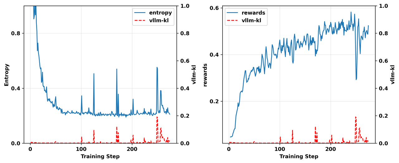
The floor also responds to the size of the update (Beyond Precision), so it is part of the optimization, not a fixed numerical error.
3. The data clock
Compare runs after the same number of rollouts. Then two settings keep three invariants.
Grow the batch by $\kappa$. With $m_u$ and $C_u$ the mean and covariance of one update before the learning rate, the first two invariants are per rollout:
$ \mathcal{A}_B = \frac{\eta\, m_u(B)}{B}\ \ (\text{progress}), \qquad \mathcal{D}_B = \frac{\eta^2 C_u(B)}{B}\ \ (\text{noise}), \qquad \text{drift} \approx \tfrac12\Big(\mathbb{E}[S^2]\,\|\mathcal{A}_B\|_F^2 + \mathbb{E}[S]\,\mathrm{tr}\big(F\mathcal{D}_B\big)\Big). $
The drift, which is the staleness term of the gap in KL units, depends only on these two and on the age $S$ of each token in rollouts. That age is the third invariant. Here $F$ is the Fisher metric, the policy’s local sensitivity. A queue configured in updates is $\kappa$ times more rollouts deep at the larger batch, so it breaks this invariant. A queue configured in rollouts keeps it:
| Setting | Rule when $B \to \kappa B$ | Keeps |
|---|---|---|
| Learning rate | $\eta \to \kappa\eta$ (SGD) or $\sqrt{\kappa}\,\eta$ (noise-dominated Adam) | Progress and noise per rollout |
| Queue | Fixed at $N$ rollouts; prefetch depth in updates $\div\,\kappa$ | The age of every token, in rollouts |
The exponent of the learning-rate rule depends on the optimizer, not on the queue:
Where the rule stops. Anything else counted in updates changes meaning when the batch grows. The momentum window spans $B/(1-\beta_1)$ rollouts, so the rule needs $N \gg \kappa B/(1-\beta_1)$. Otherwise the updates a token waits through all point the same way and the drift grows like the square of its age. The fix is to keep that window fixed in rollouts as well: $\beta_1 \to \beta_1^{\kappa}$. Coordinates dominated by signal rather than noise ask for the linear rule even under Adam, so the invariants hold on average and no better.
4. The pull at scale
A KL pull toward the sampler is a pull toward the trainer’s own past, and an age weight can make it equal at every age.
Without a weight, the pull grows like the square root of the drift, so the oldest and least trustworthy tokens pull hardest. Weighting each token’s KL by a power of its age flattens the pull exactly when the power is half the drift exponent. And because the weight counts age in updates, $\beta$ has to follow the batch:
$ w(a) = a^{-\rho},\quad \rho = p/2; \qquad \beta(\kappa B) = \kappa^{-\rho}\,\beta(B). $
With no age weight, $\rho = 0$ and $\beta$ stays fixed. The pull is delayed feedback toward past weights. It stays stable while the step size times $\beta$ times the KL curvature is well below one, and that margin shrinks as the batch, and with it the step size, grows.
5. What is derived, and what is measured
The analysis derives the shapes: the form of the update, the form of the gap, and how the step size, the queue, the momentum window and $\beta$ move together. The constants (the floor, the staleness coefficient and the exponent $p$) are local, so they have to be measured along every run with cheap gauges:
| Gauge | What it tells you |
|---|---|
| Sampler–trainer KL, by token age | The floor, and the staleness slope and exponent |
| Age histogram, in rollouts | Whether the queue really holds the age fixed |
| Update mean and covariance at two batch sizes | Whether the learning-rate rule keeps progress and noise per rollout |
| Gradient on fresh against stale data | Whether staleness has started to bend the update |
The same gauges tell you when a run has left the regime where the rule holds.
References
- J. Liu, Y. Li, et al. When Speed Kills Stability: Demystifying RL Collapse from the Training-Inference Mismatch. Blog, 2025.
- Y. Zhang, Y. Li, et al. Beyond Precision: Training-Inference Mismatch is an Optimization Problem and Simple LR Scheduling Fixes It. arXiv, 2026.
- Y. Li, J. Liu, et al. Trust Region Masking for Long-Horizon LLM Reinforcement Learning. ICML 2026.
- P. Goyal, P. Dollár, R. Girshick, et al. Accurate, Large Minibatch SGD: Training ImageNet in 1 Hour. 2017.
- S. Malladi, K. Lyu, A. Panigrahi, S. Arora. On the SDEs and Scaling Rules for Adaptive Gradient Algorithms. NeurIPS 2022.
Citation
@online{li-2026-offpolicy-gap-at-scale,
 title = {Keeping the Off-Policy Gap Fixed as RL Scales},
 author = {Li, Yingru},
 year = {2026},
 month = oct,
 url = {https://richardli.xyz/post/offpolicy-gap-at-scale/}
}

 点赞
点赞 收藏
收藏 点踩
点踩 分享
分享