Large to Small Model Stitching Destroys What You Built It to Carry Along the Fit

Independent research; early stage. Posting for feedback, particularly on whether the effect survives at realistic scale, and on prior work I've missed.

Model stitching is extensively used in AI Safety infrastructure in reusing SAE & probes to make interpretability cheaper; transferring refusal, steering vectors so that small model can help align larger ones, cross architecture model diffing (1, 2).

In this post, I expand on Chen's et al. work on Model Stitching to transfer linear features across language models. They fit affine map (a.k.a. bridge in this article) between the residual streams of smaller and larger models, using a bidirectional loss with inversion weighted by α =1; trained to convergence, the usual practice. This work zooms in on findings of feature transfer from large to small along the fit where large model's surplus retention peaks early, then declines till final checkpoint. However, geometric similarity metric is blind to this trend, and it keeps rising through the fit. This is consistent across 3 different bridge objective (one directional MSE, Cosine loss and bidirectional MSE loss at α =1) and across the hook points, which indicates fitting a bridge to convergence might start to shed what you built it to carry. This article further presents what prevents this decline using bidirectional MSE objective is the component that preserves large model's advantage by forcing reconstruction, which is underweighted with default α =1 in my toy scale setup (two 4-layer char-level GPTs, 12.7M (width: 512) and 0.21M (width: 64) params referred as and model respectively). This balance roughly depends on the ratio of variance in model's activations, which is ~4.8 in current setup.

If this effect survives realistic scale, using the bridge that fits well at convergence can lead to silent failures, as the information we aim to transfer may be partly gone. Next step is to find answer to "What it is that we gain if we stop early with default α =1 or use a balanced loss components that preserves large model's surplus while matching to small model's space?". Looking for feedback before I invest compute on training SAEs & evaluating features along the fit.

Findings in Detail

I froze both large and language models, and tracked what the bridge actually transfers through the fit, and not just at the end. Two findings:

1. Functional transfer peaks early then collapses, geometric alignment is blind to that.

• Surplus of large model through the bridge peaks early (roughly 4%) through the fit & then falls measured using probe trained on bridge along the fit, but geometric similarity metrics keeps rising. This trend appears in 3 different setup of: in bidirectional MSE loss at published α =1 and in one directional MSE & Cosine loss (for completeness). This trend appears not only when a probe is trained on bridge along the fit (upper bound of 's surplus available to extract) but also when bridge output is read through target's model frozen readout. This pattern is consistent across hook points at which bridge was trained.
• Bridges whose functional transfer metric differ by significant margin, their geometric similarity metric sits on top of each other.

(tested across 3 different bridge architecture; single seed)

Takeaway: Evalaute if you need to stop early by tracking functional metrics: retrained retention (how much XL's surplus info is there), frozen retention (how much of that is extractable in XS's space) and stitched retention (can downstream XS computation use it), along with geometric similarity.

2. Cyclic objective used by Chen et al's prevents the decline, but only if component that preserve surplus carries enough weight.

• At published α=1, decline is halved compared to one directional objective - depending on model size differences which leads to gap in activation variances ('s is ~4.8 times larger), component that defends against losing 's advantage is still down weighted. Raising α, or rescaling both streams, removes the decline while maintaining geometric similarity.
• Increasing α is not a free lunch, it does buy XL retention but the bridge stops being in basis. Across 4 different α settings, retention (calculated using retrained probe on the bridge) is almost linearly correlated with how much of survives the round trip at final checkpoint.

(tested across 3 different α settings and 1 scaled at α=1; 3 seeds)

Takeaway: If you are using Cyclic objective, check the effective weight based on models activation variance rather than trusting α=1. In this setup, balance needed α ≈ 4.8.

Metrics

This article tracks 2 set of metrics: (1) Functional transfer, indicates how much of what XL knows and XS doesn't survives? (2) Geometric alignment, captures if bridge landed in target model i.e. XS's basis? please check the detailed formula here:

Functional Transfer metrics captures how much of what XL knows and XS doesn't survives the trip, which is measured by retained %:

where, denominator is performance advantage of over , and numerator bridge performance advantage over . Ratio is the fraction of advantage that survives.

: loss of 's own readout on its activations; : loss of 's own read on its activations; computed by training standalone probes at hooked layer; : loss of readout R on bridged activations. I report 3 variations of this metric

Geometric Alignment metric captures if bridge landed on target model i.e. XS's basis? but we observed that cosine similarity is bloated as directions in transformer residual stream is anisotropic (new concept - I learned from Claude while trying to understand ~0.9 cosine similarity achieved while training one directional loss function in first attempt). To mitigate that I present Sim above shuffle and Centered similarity metrics that removes anisotropy baseline:

(generated above latex equations using Claude)

Interpretation:

• Functional transfer of 100% can drive geometric alignment to 0% - meaning bridge was able to condense all of XL's advantage into XS's dimension, but failed to keep the bridge in XS's space, where you have your interpretability tools and probe to reuse on larger model.
• Geometric alignment is 100% can lead to 0% functional transfer- meaning bridge is very closely aligned with XS's basis but lost all of XL's advantage.

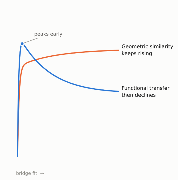
Image above depicts general trend in functional transfer and geometric alignment metrics of the bridge between large to small language models along the fit.

[Finding #1] Functional Transfer peaks then collapses; Geometric alignment is blind to that

Tested architecturally 3 different Bridge configuration and objectives for completeness.

Cosine

Bridge Architecture: Linear(, , bias=False) → LayerNorm()

Objective: (1 − cos(, ())).mean()

MSE

Bridge Architecture: Linear(, , bias=True)

Objective:

Cyclic MSE

Bridge Architecture: = Linear(, , bias=True); = Linear(, , bias=True)

Objective:

from Chen et al (equation 3), where A corresponds to and B corresponds to

Plots below present the findings from all 3 different bridge configuration that were fit after LayerNorm of transformer's final layer:

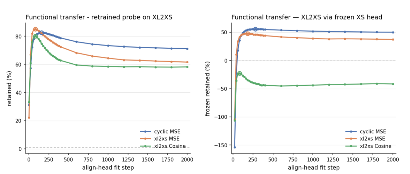
Findings:

1. Retrained Retention peak then decline is identical across different bridge architecture and objective. Both one directional Cosine and MSE peaks at step 80 and then decline; even Cyclic MSE at published α = 1 shows this trend, however the decline is halved as in cyclic loss helps preserve which is pure loss in one directional loss function. Figure 1 (c) and (d) barely show any difference in geometric similarity, sitting on top of each other. This patter indicates that it isn't Bridge architecture but a property of MSE centric objective - which is variance weighted.
2. best fit bridge at the peak, loses the most with highest peak of 85.2% @ step 80 sheds 23.6 points, not the best candidate at final checkpoint.
3. Frozen Retention follow same trend, indicating peak and decline is not an artifact of fresh retrained probe on the bridge, and XL's advantage is being lost during the fit. Frozen retention peaks a little slow & late than retrained one and the decline is less too. 47.8% (@ step 180)->37.2% for one directional MSE and 55.9% (@ step 280)->50.2% for cyclic bridge with α = 1. In order to have decent readout using target model XS tool, the bridge needs to be in XS space and increasing geometric similarity along the fit might slow it down and delay the peak somewhat.
4. Frozen Retention achieves ~50-56% of ’s advantage with no retraining, indicating a good chunk of what knows beyond is expressible inside ’s own readout directions as well.
5. Geometric Alignment metric can’t see the difference. All 3 bridges plateau at cosine-above-shuffle ≈ 0.62, and their curves are visually superimposed along the fit. Meanwhile functional transfer follows an entirely different trend with metrics differing by several points at peak and at final checkpoint. Any practitioner watching geometric similarity would see all three bridges as equivalent and would completely miss the peak and settle with the bridge where it has already shed sparse features.

Why peak then collapse?

Gradient descent on MSE loss, resolve high variance directions first before getting to sparse ones. Dominant directions are may be shared between source and target model, but in a superimposed way (due to polysemanticity). Early in the fit (see figure1 (a) & (c)) both retrained retention and sim above shuffle rises together, transferring these dominant directions first which takes superimposed features along with it. What happens to XL's surplus next depends on the objective function:

• One directional objective treats anything that's not in XS's space as pure error. After the peak it may spend rest of the training separating these superimposed direction and getting ride of surplus, converging towards least squared predictor of XS. But the trade seems unbalanced, from its peak (step 80) to the end of the fit, cosine-above-shuffle rises by only 0.08 (0.54 → 0.62), while retention falls by 23.6 points (85.1% → 61.5%).
• A cyclic consistency term in the loss function the changes this pattern, because not able to reconstruct XL adds to error as well that makes retention of XL's surplus critical. How much of the collapse it prevents turns out to depend on a weighting between these opposite forces of match to XS space and XL reconstruction (Finding #2).

[Finding #1.2] Bridge hook point doesn't change the story

Midway through my experiments I realized the hook point in Chen et al. (2025) was different from what I had started experimenting with (final layer post ln), so I took one directional MSE loss and started training & evaluating bridge across 3 different hook points in parallel: Final layer post-LayerNorm, final layer pre-LayerNorm and residual stream entering third layer, and this is how above metrics through the fit:

Findings:

1. Retrained retention early peak and decline trend is consistent across the hook points. Retention % is showing a significant gap between final layer and mid layer of 56 points (74.6% vs 18.6% -> ~4times gap), however in absolute terms bridge transfers 0.27 nats vs 0.15(~2 times gap).
2. Frozen retention has no peak for bridge hooked mid depth and its only able to retrain 2% of XL's advantage when read through frozen target model's readout.
3. Geometric Similarity is maximum for bridge hooked mid depth; again expected as it closer to input and residual variance is dominated by input drive dominant features, as training data is shared between models.

[Finding #2] Cyclic Bridge prevents the decline only if the component that preserves surplus carries enough weight

Setup. Following Chen et al. (2025), the cyclic bridge that learns a linear down-map () and an up-map (), trained with objective

They published α = 1 by running ablation over α by evaluating downstream next-token cross entropy loss (aligned with stitched retention that article reports) and loss of SAE transfer from A to B (small to large in this setup - which I haven't done yet - listed as one of the follow-ups below) - where at this value all the metric loss were low at once.

The underlined components play a critical role in large to small bridge: (i) component is responsible to reconstruct back from bridge output in 's dimension, and must contain what knows including what lacks. Whatever discards shows directly as error. (ii) anchors the bridge in XS's space and any XL's surplus contributes to error. α sets which force wins. As we noticed merely introducing with equal weight i.e. α = 1 halves the decline, by preserving more of XL's surplus compared to one directional ones after peak, but the question is can we avoid the decline w/o sacrificing geometric alignment? Plots below answers that:

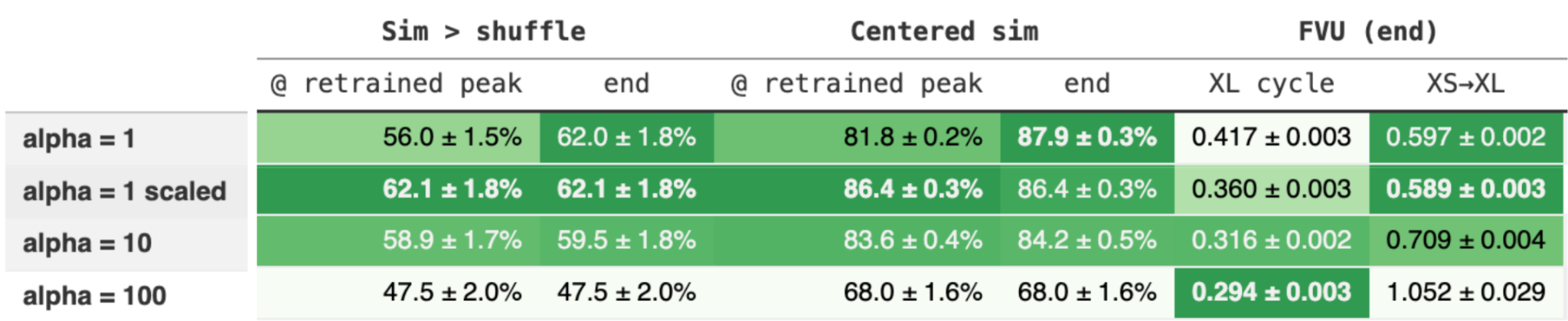
As α rises:

• The decline disappears & retention keeps rising; see retrained retention figure1 (a) as α=1 retrained retention drops by 11.4 points, but at α=10 it plateaus ~9 points higher and even higher for α=100.
• More of XL survives the bottleneck; supported by cycle FVU metric, the fraction of 's variance lost through the round trip , falls monotonically.
  
• Geometric alignment goes down; sim above shuffle declines from ~62% at α=1 to ~59% at α=10 to ~46% at α=100, while highest retrained retention made a jump from 82.6% to 94.4% for α=1 to 100. Indicating even though more of survives the roundtrip, it aligns less and less with space. Another artifact to the wider phenomenon of representational similarity diverging from functional.

Why α=1 is weaker? For any MSE, it is equal to Variance of target space times FVU. Now, when we apply that 2 terms that pull against each other

• = ; any 's surplus is adds to error
• = ; any loss in 's retention adds to error

During gradient descent, one unit of 's reconstruction FVU costs and one unit of to matching FVU costs . The effective weight of preserving while maintain match to is .

At post-ln_f, and . Balance () therefore needs , and the default α=1 gives indicating reconstruction is downweighted, which explains sustained peak then decline in functional transfer at α=1 for the experiment setup used here.

*Not converged at step 2000.

Scaling activations to unit RMS achieves the balance in other way but same concept at α=1. At post-ln_f, and ; ratio of is roughly equal to ~4.8.

Retrained and frozen retention disagree past balance A retrained probe only needs the information to be present. A frozen probe needs it in the directions 's own readout uses. Frozen retention is highest near balance: scaled α=1 reaches 67.5% and α=10 achieves 66.3%, against 50.2% at default α=1. Pushing further collapses it. At α=100 frozen retention is −33.1% while retrained retention is 94.3%, the highest of any bridge.

This indicates XL's retention and landing on XS's space can strike a optimal balance when both components in loss function is weighted equally.

Experiment Setup

Models [code]: Two char-level miniGPTs trained on TinyStories (327M characters; unigram entropy 3.07 nats).

• XS: width 64, 0.21M parameters, eval loss 1.039 nats (avg. across 3 seeds)
• XL: width 512, 12.7M parameters, eval loss 0.674 nats (avg. across 3 seeds)

Shared model training configs (pasted below), trained using AdamW till convergence and frozen for everything that follows.

train_config = {
 'vocab_size' : 62,
 'block_size' : 128,
 'n_heads' : 4,
 'n_layers' : 4,
 'dropout' : 0.1,
 'batch_size' : 64,
 'lr' : 3e-4,
 'max_steps' : 40000,
 'eval_every' : 250,
 'grad_clip' : 1.0
}

Bridge hook sites: bridges are fit at one of these sites:

• final layer; post LayerNorm: activations are used as-is.
• final layer; pre LayerNorm: activations are divided by its RMS over eval batch.
• residual stream entering; third block out of 4 layers (block2): activations are divided by its RMS over eval batch.

W/o scaling pre LayerNorm at existing lr, bridge was converging far more slowly. I experimented with larger lr for these sites, but training look longer, comparing along the fit was getting messy and less obvious (I still need to do a bit more digging here). For finding #1.2, the post-ln_f bridge is also run scaled, so the three sites are compared like for like. And that's how I stumbled upon scaling solution within Cyclic loss setup.

Bridge [code]: All bridge maps (512)-> (64). Weights are initialized N(0, 0.02) with zero biases. Each is trained for 2,000 steps with AdamW (lr 1e-3, PyTorch's default weight decay of 0.01) on fresh training batches with trajectory config below.

traj_config = {
 'align_steps' : 2000,
 'snap_every' : 200,
 'snap_early_until' : 400,
 'snap_early_every' : 20,
 'probe_steps' : 2500,
 'probe_seed' : 1234,
 'lr': 1e-3
}

The bridge is saved every 20 steps up to step 400, then every 200 steps to step 2,000. All metrics are computed on every snapshot.

Probes [code]: Bias free linear map from activation to next character logits.

• Standalone probes on XS and XL are needed for denominator for functional transfer metric
• Fresh probe is trained on the bridge at every step to calculate retrained retention: upper cap XL's surplus that was transferred.

All probes are trained with probe seed: 1234.

Evaluation. All losses and geometry are measured on the same 10 fixed evaluation batches (eval seed 999).

Immediate FollowUps

• Validate if these findings survives realistic scale models.
• Retrain model & bridge with BPE tokenizer instead of Char, and run α configuration to see if Finding #2 holds true. Supplement the findings by training SAEs on target model and reusing onto bridge, evaluating along the trajectory to check which surplus features are being shed during decline after peak.
  Helps answer the question "What it is that we gain if we stop early while training with default α =1 or use a balanced loss components that preserves large model's surplus while matching to small model's space?"
• I have used single seed for Finding#1 due to compute constraint, and spend the resources on 3 seeds to solidify Finding#2, personally I find that more critical. Happy to hear more opinions on the experiment setup.

Please suggest more. Thank you very much for reading!