Aperiodic tilings with the de Bruijn method
A couple of weeks ago I wrote a somewhat earnest post warning about some of the difficulties you can encounter when using the dplyr::ntile() function to construct quantile-based groups in R. I was somewhat pressed for time, but still wanted to follow my usual practice of including “interstitial” graphics, which I usually do by repurposing my own hand-written generative art code to create nice looking horizontal separators. As I said, I was pressed for time, so rather than using my own code, I used an R translation of the samacqua/tilings Python/matplotlib repository, which applies the de Bruijn grid method for generating aperiodic rhombus tilings (…because the function is called n-tile, and we can make the images from n tiles, gosh I’m soooo clever aren’t I???????)
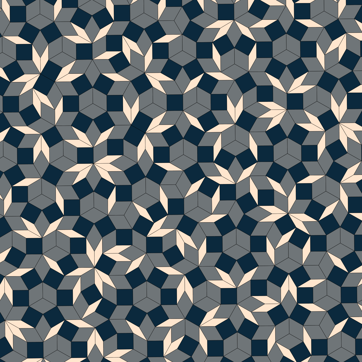
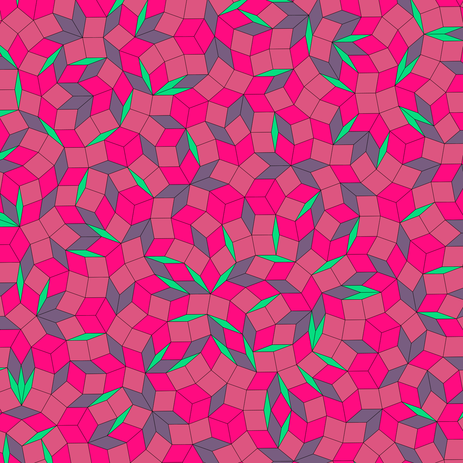
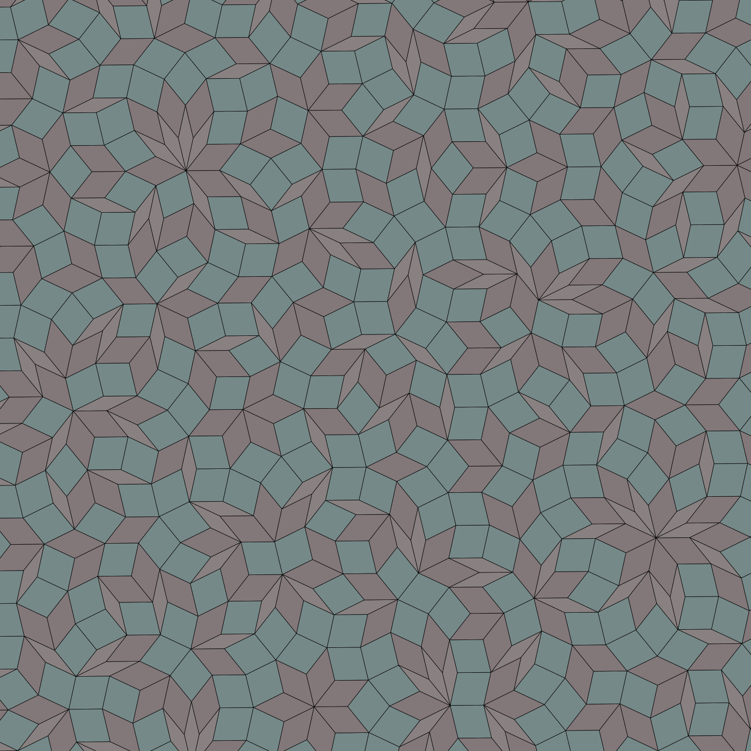
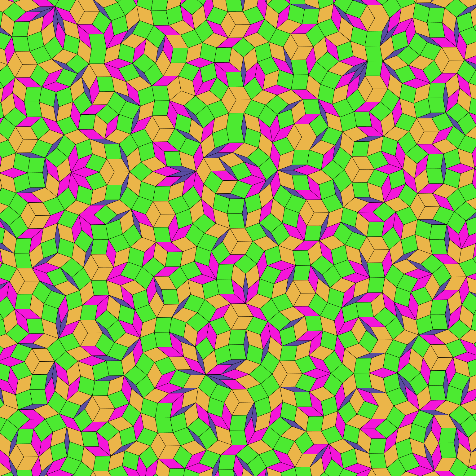
The images you can create using this method are really quite lovely:
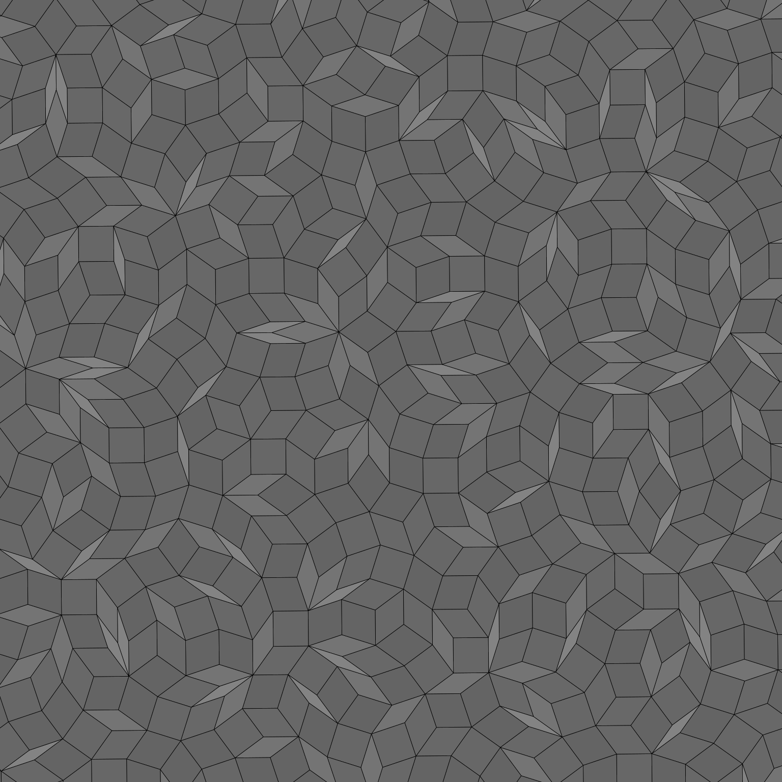
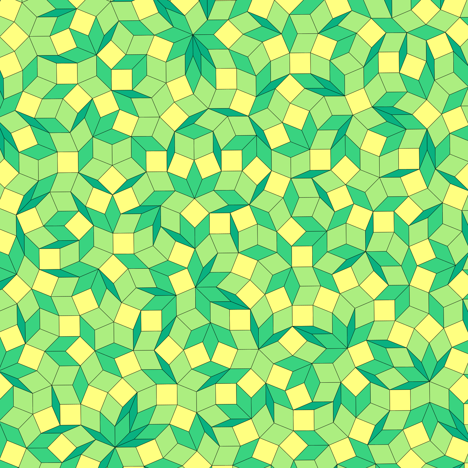
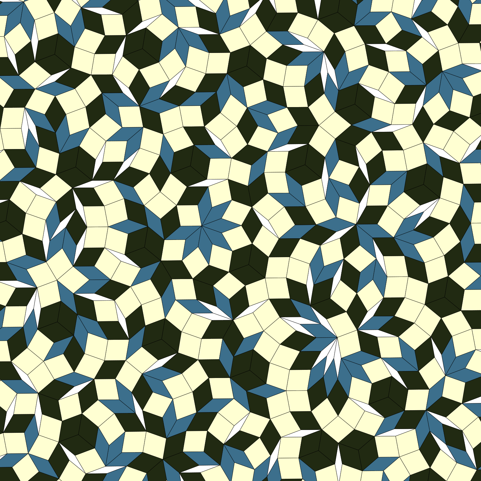
I love these enough that I’d like to use them to make my own artwork. The rigid geometric style isn’t usually my preferred way to make generative art, since my personal tastes lean to more flowing pieces, but even so it’s a technique I’ve used in the past (e.g., here and here) and often think I ought to play around with it more.
However. For these de Bruijn tilings, I have a problem. I didn’t write the code myself. The mathematical methods underpinning the tilings come from a 1981 article by N. G. de Bruijn; Sam Acquaviva wrote the Python library, and because I was under time pressure to wrap up the blog post I can’t even take credit for the R translation because I was in a rush and asked Claude to do it for me. At the time I made the first batch of figures (the ones used in the ntile blog post) I didn’t even have a very good grasp of what the code was doing. All I’d done was skim some of the references, take a brief look at the code Claude threw at me, and made some pretty pictures.
In no sense of the term was this my own code, much less my own art. Nothing in that production process involved me thinking much about either the code or the art. In complete honesty there’s very little difference between what I did to create those tilings and what talentless hacks do when they type a prompt into Midjourney, get it to spit out an image, and then say they made the art themselves. They absolutely did not. There’s zero artistic merit in that process1 and frankly there wasn’t any more merit involved in mine.
Part of what is missing, in both cases, is genuine understanding of the process. What’s missing when people make the “my child could have made this” critique of art they don’t like – thinking that it lacks skill – is recognition of a fundamental difference between an artist who understands the craft making a choice to employ a style, and someone creating the same output with zero understanding. In art, the method of production matters. The artist is not completely separable from the art, and if the artist doesn’t know what they’re doing they can’t make a strong claim to authorship (in my opinion).
But… goddamn it I love these tilings and I want to use them. And so with that in mind I’ve decided to make amends for my rushed artistic faux pas. The original R translation that Claude created was written entirely in base R, plus a small amount of ggplot2 to take care of the final plotting step. It works, but I didn’t like the way the code reads. I find tidyverse style easier to read, and I tend to understand what it does more easily than code written in the base R style. So what I decided to do was rewrite Claude’s base R code myself adopting the tidyverse style, and annotating the code with my own comments on what it does.
Compared to the effortless speed with which Claude could have done much the same thing – for like $2 at most – the manual rewrite was slow and painful. But something important came out of doing it that way: this time around I genuinely understand the code. I know what it does. I can explain it to others. I understand de Bruijn tilings much, much better now than I did before, and this understanding gives me the capacity to make real artistic choices in how I use this technique later on.
This matters to me. I am not fundamentally opposed to the machines – I am not threatened by the fact that I cannot outrun a car or outlift a crane. Indeed, apart from my practical economic anxieties (I rather like having a job, thank you very much) I’m not even all that concerned that LLMs can code faster and probably better than I can. But I am concerned about atrophy. If I rely too much on cars my fitness evaporates.2 If I don’t do strength training from time to time I become vulnerable to injury. Delegating the manual labour work to the machine has serious physical side-effects, and it is no different for cognitive labour. If you let the machine do your thinking for you, your capacity to think for yourself withers and dies. If you let it make your art, you lose your artistic skills. I am not willing to accept that outcome. It’s bad enough that I can feel the cursed machines dulling my thoughts at work because I’m being pushed to use them professionally. But to have them steal my soul in the process? Nope. Fuck right the fuck off with that.
So… with that as my artistic preamble, let’s talk about de Bruijn tilings.
library(ggplot2)
library(tibble)
library(purrr)
library(tidyr)
library(dplyr)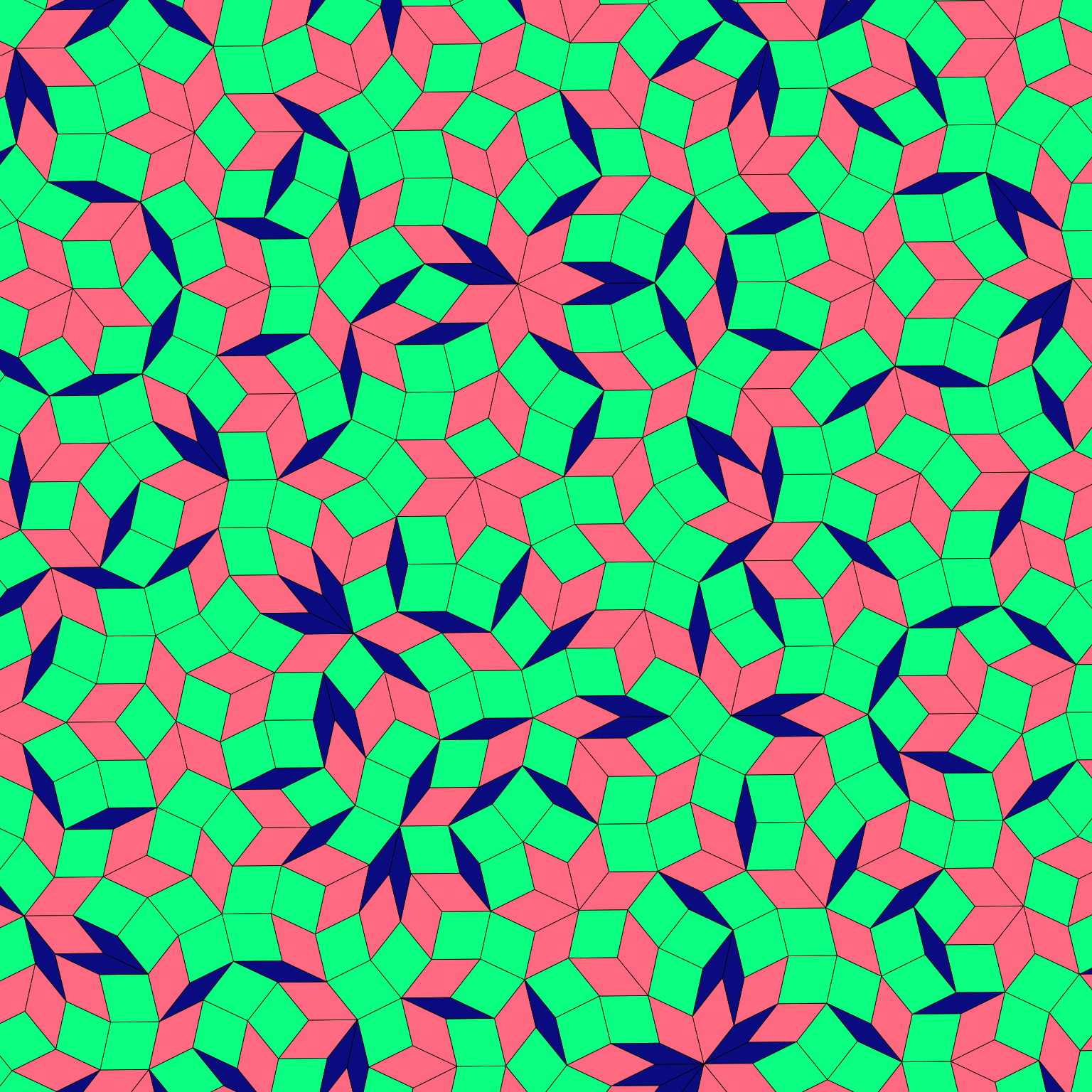
Defining a rhombus from an intersection
The place to begin any discussion of de Bruijn tilings is with the observation that the key “trick” is to define several families of parallel lines, and at every location where lines from different families intersect, we define a rhombus whose edges are orthogonal to the intersecting lines. This feature creates a critical property: any two rhombi that sit on the same line will have edges that are parallel to one another, and can be placed adjacent to each other in a tiling. In the simplest approach to aperiodic tilings via the de Bruijn method, all we end up doing is glueing these rhombi to one another one by one (more on that later). The original paper goes somewhat deeper and shows that you can construct Penrose-style “kite and dart” tilings from these rhombi, but I won’t talk about that extension here. We’re all about the rhombi in this post.
So, given that the “rhombi from intersections” trick is central to how de Bruijn tiling works, the natural place to start building the code is with a suitable build_rhombus() function: the user specifies information about the intersection and the function outputs the corresponding rhombus. There are four critical arguments to this function:
x_midandy_midare used to specify location of the intersection, which becomes the centroid of the rhombus once it is constructed.angle_1andangle_2are used to specify the orientation of the two lines that form the intersection (in radians, not degrees).
The other arguments aren’t needed right now: they supply additional bookkeeping information that is useful when the tiling is assembled, but the build_rhombus() function itself treats them as metadata and doesn’t do anything interesting with them other than pass them directly into the output object. Here’s the code:
# Every intersection of two grid lines becomes a rhombus, in the usual
# "dual" construction for these grid methods: the rhombus edges run
# perpendicular to the two line directions that cross at this point, and
# its two pairs of opposite edges have length `2 * scale`.
build_rhombus <- function(x_mid,
                          y_mid,
                          angle_1,
                          angle_2,
                          offset_1 = NA_real_,
                          offset_2 = NA_real_,
                          family_1 = NA_real_,
                          family_2 = NA_real_,
                          line_1 = NA_real_,
                          line_2 = NA_real_,
                          scale = 1) {

  # Rhombus edge directions are rotated 90 degrees from the line angles;
  # this ensures that rhombi that sit on the same line will have matching
  # faces, and can be tiled next to one another without gaps when the
  # tiling is assembled
  rh_angle_1 <- angle_1 + pi / 2
  rh_angle_2 <- angle_2 + pi / 2

  # These are unit vectors pointing along the two pairs of edges
  d1 <- c(-sin(rh_angle_1), cos(rh_angle_1))
  d2 <- c(-sin(rh_angle_2), cos(rh_angle_2))

  # Centroid coordinates as a named vector; names become the column names
  # for the vertices matrix, and later become column names for the data
  # frame
  centre <- c(x = x_mid, y = y_mid)

  # The four corners, reached from the centre by moving +/- scale along
  # each of the two edge directions in turn; it is convenient to represent
  # vertices as a matrix rather than a data frame, even though plotting is
  # easier in the latter format.
  vertices <- rbind(
    centre + scale * d1 + scale * d2,
    centre - scale * d1 + scale * d2,
    centre - scale * d1 - scale * d2,
    centre + scale * d1 - scale * d2
  )

  # The angle *between* the two grid-line directions determines the shape
  # of the rhombus (a 72-degree gap between line families gives "thin"
  # Penrose rhombi, a 36-degree gap gives "fat" ones, etc). Reducing this
  # angle to its smallest equivalent (the acute angle, <= pi/2) gives a
  # single number that identifies the tile's shape regardless of its
  # orientation: it's not strictly needed to construct the tiling, but gets
  # used later to decide the fill colour of a tile
  diff <- abs((rh_angle_2 - rh_angle_1) %% (2 * pi))
  if (diff > pi) diff <- 2 * pi - diff
  tile_acute <- if (diff > pi / 2) pi - diff else diff

  # Return the built rhombus as a list containing a matrix of vertices,
  # plus a one-row tibble of metadata: the acute angle (for colouring)
  # and, crucially, *which* two grid lines (family + line index) this
  # tile sits on. Keeping track of this is critical for the tiling process,
  # since compute_neighbours() and build_tiling() later match tiles up by
  # looking for shared (family, line) pairs
  list(
    vertices = vertices,
    properties = tibble(
      tile_acute = tile_acute,
      x_mid = x_mid,
      y_mid = y_mid,
      angle_1 = angle_1,
      angle_2 = angle_2,
      offset_1 = offset_1,
      offset_2 = offset_2,
      family_1 = family_1,
      family_2 = family_2,
      line_1 = line_1,
      line_2 = line_2
    )
  )
}
To illustrate this, let’s create a rhombus defined by two lines, one oriented at 45 degrees counterclockwise from north (the red line below, which points northwest in map coordinates) and the other at 120 degrees from north (the blue line below). In hindsight I’m not sure if I would have defined the angles using “radians counterclockwise from north” as the unit, as I am much more accustomed to thinking about angles as “radians counterclockwise from east”, but that’s how it was set up in the code I inherited and it’s not doing any harm, so I left it as-is:
rh <- build_rhombus(
  x_mid = 0,
  y_mid = 0,
  angle_1 = pi / 4,     # 45 degrees
  angle_2 = 2 * pi / 3  # 120 degrees
)
rh
$vertices
x y
[1,] -0.2071068 -1.5731322
[2,] 1.2071068 -0.1589186
[3,] 0.2071068 1.5731322
[4,] -1.2071068 0.1589186
$properties
# A tibble: 1 × 11
tile_acute x_mid y_mid angle_1 angle_2 offset_1 offset_2 family_1 family_2
1 1.31 0 0 0.785 2.09 NA NA NA NA
# ℹ 2 more variables: line_1 , line_2 As described above the data structure is a matrix of vertices and a tibble containing useful metadata properties for the rhombus. Here’s what it looks like plotted:
# Convert a "radians counterclockwise from north" angle into a
# slope that can be interpreted by geom_abline()
as_slope <- function(angle) {
  dx <- -sin(angle)
  dy <- cos(angle)
  dy/dx
}

# The two data frames needed for the plot
vt <- as_tibble(rh$vertices)
pr <- rh$properties

# The plot itself
ggplot() +
  geom_polygon(aes(x, y), data = vt, fill = "snow", color = "black") +
  geom_abline(slope = as_slope(pr$angle_1), intercept = 0, color = "tomato") +
  geom_abline(slope = as_slope(pr$angle_2), intercept = 0, color = "slateblue") +
  coord_equal(xlim = c(-2, 2), ylim = c(-2, 2)) +
  geom_point(aes(x_mid, y_mid), data = pr, size = 3)
The orientation of the rhombus relative to the red and blue lines looked visually jarring to me when I first started reading about de Bruijn tilings, but the diagram makes more sense when you look closely. Every time the red line or the blue line crosses one of the edges of the rhombus, it is always at a 90 degree angle. That’s central to the de Bruijn tiling procedure, and the key design feature of the build_rhombus() function.
Defining families of grid lines
Now that we have a method for placing rhombi on an intersection, we need the ability to construct the grid lines and intersections that the de Bruijn method uses to define the set of to-be-tiled rhombi. Let’s say we want to construct a de Bruijn tiling with n_families = 5 sets of parallel lines. Each set of lines is oriented at a specific angle (again, measured in radians counterclockwise from north), and displaced horizontally from the origin by an offset value. These offsets are important, but for the moment we’ll ignore them.
The build_families() function below is used to set up the line families:
# There's no probabilistic component to setting the angles that define
# the line families; only to the horizontal offsets that displace them.
# The default value to `angle_offset` is deliberately slightly non-zero,
# which means that angles are not *strictly* defined relative to north,
# but are ever so slightly rotated. This is purely a numerical convenience,
# to avoid issues that pop up with vertical lines (infinite slope)
build_families <- function(n_families,
                           offsets = NULL,
                           angle_offset = 0.01,
                           seed = NULL) {

  # if the line family offsets aren't set, generate them randomly
  if (is.null(offsets)) offsets <- sample_offsets(n_families, seed = seed)

  # return a tibble with summary information for each line family
  tibble(
    family  = seq_len(n_families),
    offset = offsets,
    angle  = (family - 1) * pi / n_families + angle_offset
  )
}
Here’s what we obtain for three families with no offsets:
fam <- build_families(n_families = 3, offsets = c(0, 0, 0))
fam
# A tibble: 3 × 3
family offset angle
1 1 0 0.01
2 2 0 1.06
3 3 0 2.10It’s a little easier to see this in the form of a plot. In the image below I’m only showing one line for each family. When we get to the stage of seeing the full grid of lines, each line within a family will be assigned an index: what we’re looking at below is the special case when the indexing value is zero, and when there are no offsets applied. The consequence is that all the lines pass through the origin:
show_families <- function(fam) {
  fam |>
    mutate(
      family = factor(family),
      dx = -sin(angle),
      dy = cos(angle),
      x1 = -dx + offset,
      x2 = dx + offset,
      y1 = -dy,
      y2 = dy,
    ) |>
    ggplot(aes(x1, y1, xend = x2, yend = y2, color = family)) +
    geom_segment(linewidth = 1) +
    coord_equal()
}

show_families(fam)
Although this is the simplest scenario, it’s genuinely undesirable for a de Bruijn tiling. When creating these tilings, we want to preserve the exact one-to-one mapping between intersections and rhombi. Any time that three or more lines pass through the same point this mapping breaks, which is the reason why we introduce the horizontal offsets that displace each of the line families in a way that prevents this from happening. The sample_offsets() function below does this for us: it enforces the constraints that two families cannot share the same offset value, and no two offsets can sum to a whole number. This is what prevents three or more lines from ever intersecting:
# Each of the line families is offset horizontally from the origin by a phase
# These phases are what make the resulting tiling look "random"
sample_offsets <- function(n_families, eps = 1e-6, seed = NULL) {
  if (!is.null(seed)) set.seed(seed)
  offsets <- runif(n_families)
  repeat {
    bad <- outer(offsets, offsets, function(a, b) abs(a - b) < eps) |
      outer(offsets, offsets, function(a, b) abs(a + b - 1) < eps)
    diag(bad) <- FALSE
    if (!any(bad)) break
    idx <- which(rowSums(bad) > 0)
    offsets[idx] <- runif(length(idx))
  }
  offsets
}
Here’s an example of that. The build_families() function defined earlier is designed so that if the user doesn’t manually specify offsets, it uses the sample_offsets() function above to generate them randomly:
fam <- build_families(
  n_families = 3,
  offsets = NULL,
  seed = 1
)
show_families(fam)
This version is more suited to our purposes: it avoids the degenerate case where three lines meet in a point, and it would be possible to uniquely call the build_rhombus() function separately from each of the three intersections shown in the plot. We can’t literally do that yet because I haven’t built the function that detects the intersections and tags each intersection with the relevant line angles, but that’s coming!
Using the families to build out the grid
Now that we have the basic idea for line families in place, we’ll define a build_grid_lines() function that approaches it a little more systematically. Here, the user passes x_scale and y_scale arguments that are used to define a bounding box; build_grid_lines() detects every member of every line family that passes through that box. In this code it is implicit that the distance separating adjacent lines within the same family is always fixed at 1. Here’s the code for the function:
# Handy little infix operator to check if a scalar value falls within the
# range specified by a length-2 vector
`%within%` <- function(value, range) range[1] <= value & value <= range[2]

# Build the families of parallel lines, and populate each family with a
# sufficient number of lines to fill the bounding box (defined by the
# x_scale and y_scale parameters). Returns a data frame with one row for
# each line that passes through the bounding box, with coordinates and
# other useful information.
build_grid_lines <- function(x_scale,
                             y_scale,
                             offsets,
                             eps = 1e-6) {

  # Set up the line families
  n_families <- length(offsets)
  families <- build_families(n_families, offsets)

  # Define the bounding box; keep this internal because it's not really a
  # plot limit; it behaves like a plot limit for the purposes of this
  # function, but when the final tiling gets assembled the rhombi get moved
  # around, so the final plot limits are different
  xlim <- c(-x_scale, x_scale)
  ylim <- c(-y_scale, y_scale)

  # For each family, work out which integer `line` values could possibly
  # intersect the box at all, so later steps don't waste time clipping
  # lines that are nowhere near it. `corner_k` evaluates the line equation
  # `x*cos(angle) + y*sin(angle) + offset` at each of the box's 4 corners.
  # The resulting range of `line` must cover every integer between the
  # smallest and largest corner value (with a 1-unit pad on each side, to
  # be safe about rounding) for the family's lines to span the box
  line_cases <- families |>
    cross_join(expand_grid(xlim, ylim)) |>
    mutate(corner_k = xlim * cos(angle) + ylim * sin(angle) + offset) |>
    reframe(
      .by = family,
      across(c(offset, angle), first),
      line = seq(
        from = floor(min(corner_k)) - 1,
        to = ceiling(max(corner_k)) + 1
      )
    )

  # Function to clip one specific line (one `family`/`line` combination)
  # to the bounding box. A line can leave the box through a horizontal edge
  # (at y = ylim) or a vertical edge (at x = xlim); this solves for both and
  # keeps only the crossing points that are actually within the box
  # (`x_ok`/`y_ok`), then de-duplicates in case a line passes exactly
  # through a corner. Near-horizontal/near-vertical lines need the
  # opposite equation (division by a near-zero cos/sin), which is why both
  # cases are computed and only the valid one(s) kept via `eps`.
  build_grid_line <- function(family, offset, angle, line) {

    points <- bind_rows(
      tibble(
        y = ylim,
        x = (line - offset - y * sin(angle)) / cos(angle),
        x_ok = x %within% xlim,
        y_ok = abs(sin(angle)) > eps
      ),
      tibble(
        x = xlim,
        y = (line - offset - x * cos(angle)) / sin(angle),
        y_ok = y %within% ylim,
        x_ok = abs(cos(angle)) > eps
      )
    )

    points <- points |>
      filter(x_ok & y_ok) |>
      distinct()

    # A line that misses the box entirely contributes no segment. This
    # isn't expected to happen normally, but retained just in case
    if (nrow(points) == 0) {
      return(tibble(
        family = numeric(0),
        line = numeric(0),
        angle = numeric(0),
        offset = numeric(0),
        x1 = numeric(0),
        y1 = numeric(0),
        x2 = numeric(0),
        y2 = numeric(0)
      ))
    }

    tibble(
      family = family,
      line = line,
      angle = angle,
      offset = offset,
      x1 = points$x[1],
      y1 = points$y[1],
      x2 = points$x[2],
      y2 = points$y[2]
    )
  }

  # Clip every candidate line in every family, and return a tibble
  line_cases |> pmap_dfr(build_grid_line)
}
Here’s what it returns:
lines <- build_grid_lines(
  x_scale = 5,
  y_scale = 5,
  offsets = sample_offsets(n_families = 3, seed = 1)
)

lines
# A tibble: 38 × 8
family line angle offset x1 y1 x2 y2
1 1 -4 0.01 0.266 -4.22 -5 -4.32 5
2 1 -3 0.01 0.266 -3.22 -5 -3.32 5
3 1 -2 0.01 0.266 -2.22 -5 -2.32 5
4 1 -1 0.01 0.266 -1.22 -5 -1.32 5
5 1 0 0.01 0.266 -0.216 -5 -0.316 5
6 1 1 0.01 0.266 0.785 -5 0.685 5
7 1 2 0.01 0.266 1.78 -5 1.68 5
8 1 3 0.01 0.266 2.78 -5 2.68 5
9 1 4 0.01 0.266 3.78 -5 3.68 5
10 1 5 0.01 0.266 4.78 -5 4.68 5
# ℹ 28 more rowsThe lines tibble contains the following columns:
familyis the index for the line familylineis the index that labels a specific line within a familyanglekeeps track of the angle that defines the familyoffsetkeeps track of the horizontal offset for the familyx1andy1define one point at which the line intersects the bounding boxx2andy2define the other point at which the line intersects the box
Noting this, it’s fairly straightforward to translate this into a visualisation of the grid lines:
lines |>
  mutate(family = factor(family)) |>
  ggplot(aes(x1, y1, xend = x2, yend = y2, color = family)) +
  geom_segment(linewidth = 1) +
  coord_equal()
Every intersection in this plot will later be used to construct a single rhombus, and the tiling will be constructed by assembling these rhombi. So the next step in the process is to define a function that can detect all these intersections.
Detecting the intersections
Mechanically, detecting the intersection between a pair of lines is not difficult, as it corresponds to solving two simultaneous linear equations: high school level algebra, thankfully. The find_intersections() function below takes a data structure like lines above, and finds all the points at which an intersection occurs. The code below is a little longer than you might expect for a task this simple, but most of it is bookkeeping and overly-long comments that I’ve added purely for pedagogical purposes:3
# Find every point where a line from one family crosses a line from
# another family, within the bounding box. Lines in the same family
# are parallel, so the search is performed across pairs of lines that
# belong to different families.
find_intersections <- function(lines,
                               x_scale = NULL,
                               y_scale = NULL,
                               eps = 1e-10) {

  # Detect the box scale from the lines if the user doesn't specify
  if (is.null(x_scale)) x_scale <- max(abs(c(lines$x1, lines$x2)))
  if (is.null(y_scale)) y_scale <- max(abs(c(lines$y1, lines$y2)))

  # As before: keep this internal because it's not really a plot limit
  xlim <- c(-x_scale, x_scale)
  ylim <- c(-y_scale, y_scale)

  # Find all unique pairs of line families: the base R combn() function
  # is more efficient in general but expand_grid() then filter() is
  # perfectly fine here
  family <- sort(unique(lines$family))
  family_pairs <- expand_grid(family_1 = family, family_2 = family) |>
    filter(family_2 > family_1)

  # Helper function used to detect all the intersections between two
  # line families that fall inside the plotting area
  find_family_intersections <- function(family_1, family_2) {

    # Empty tibble to return if there is no intersection
    null_intersection <- tibble(
      x = numeric(0),
      y = numeric(0),
      angle_1 = numeric(0),
      angle_2 = numeric(0),
      offset_1 = numeric(0),
      offset_2 = numeric(0),
      family_1 = numeric(0),
      family_2 = numeric(0),
      line_1 = numeric(0),
      line_2 = numeric(0)
    )

    # Sets of lines associated with each of the two families
    line_set_1 <- lines |> filter(family == family_1)
    line_set_2 <- lines |> filter(family == family_2)

    # The angles specifying the two line families
    angle_1 <- line_set_1$angle[1]
    angle_2 <- line_set_2$angle[1]

    # The offsets associated with the two line families
    offset_1 <- line_set_1$offset[1]
    offset_2 <- line_set_2$offset[1]

    # Take sin and cosine of both angles
    cos_a1 <- cos(angle_1)
    sin_a1 <- sin(angle_1)
    cos_a2 <- cos(angle_2)
    sin_a2 <- sin(angle_2)

    # Return an empty tibble if the determinant is too low. When
    # det = 0 the lines are exactly parallel and no intersection
    # exists. A threshold is applied to avoid numerical issues
    # that arise with nearly-parallel lines
    det <- cos_a1 * sin_a2 - cos_a2 * sin_a1
    if (abs(det) < eps) return(null_intersection)

    # Determine an "adjusted" coordinate for each line, after taking
    # family-specific offset values into account; then compute the x
    # and y values at which the intersection occurs; retaining only
    # those intersections that remain within the plot limits
    grid <- expand_grid(
      line_1 = line_set_1$line,
      line_2 = line_set_2$line
    ) |>
      mutate(
        line_coord_1 = line_1 - offset_1,
        line_coord_2 = line_2 - offset_2,
        x = (line_coord_1 * sin_a2 - line_coord_2 * sin_a1) / det,
        y = (line_coord_2 * cos_a1 - line_coord_1 * cos_a2) / det,
        keep = (x %within% xlim) & (y %within% ylim)
      ) |>
      filter(keep)

    # If none of the pairs are retained return an empty tibble
    if (nrow(grid) == 0) return(null_intersection)

    # Return a tibble containing the retained intersections
    grid |>
      transmute(
        x = x,
        y = y,
        angle_1 = angle_1,
        angle_2 = angle_2,
        offset_1 = offset_1,
        offset_2 = offset_2,
        family_1 = family_1,
        family_2 = family_2,
        line_1 = line_1,
        line_2 = line_2
      )
  }

  family_pairs |> pmap_dfr(find_family_intersections)
}
This is the data structure returned by find_intersections():
inter <- find_intersections(lines)
inter
# A tibble: 265 × 10
x y angle_1 angle_2 offset_1 offset_2 family_1 family_2 line_1
1 -4.22 -4.94 0.01 1.06 0.266 0.372 1 2 -4
2 -4.23 -3.78 0.01 1.06 0.266 0.372 1 2 -4
3 -4.24 -2.63 0.01 1.06 0.266 0.372 1 2 -4
4 -4.25 -1.47 0.01 1.06 0.266 0.372 1 2 -4
5 -4.26 -0.319 0.01 1.06 0.266 0.372 1 2 -4
6 -4.27 0.836 0.01 1.06 0.266 0.372 1 2 -4
7 -4.29 1.99 0.01 1.06 0.266 0.372 1 2 -4
8 -4.30 3.14 0.01 1.06 0.266 0.372 1 2 -4
9 -4.31 4.30 0.01 1.06 0.266 0.372 1 2 -4
10 -3.22 -4.35 0.01 1.06 0.266 0.372 1 2 -3
# ℹ 255 more rows
# ℹ 1 more variable: line_2 Now that we have the locations of the intersections we can re-create the grid lines plot from before, but annotate it with points located at each intersection:
lines |>
  mutate(family = factor(family)) |>
  ggplot(aes(x1, y1, xend = x2, yend = y2, color = family)) +
  geom_segment(linewidth = 1) +
  geom_point(aes(x, y), data = inter, size = 3, inherit.aes = FALSE) +
  coord_equal()
Placing rhombi at the intersections
We now have all the parts that we need to create the rhombi and place them on top of the appropriate intersection on the grid. The code below does this, and returns a conveniently-plottable rhombi tibble:
# Repeat the grid/intersection construction with a smaller box
offsets <- sample_offsets(n_families = 3, seed = 1)
lines <- build_grid_lines(x_scale = 2, y_scale = 2, offsets)
inter <- find_intersections(lines)

# Map the intersections onto rhombi using build_rhombus(),
# extract the vertices component, and make a tidy tibble
rhombi <- inter |>
  mutate(scale = .2) |>
  pmap(build_rhombus) |>
  imap_dfr(\(r, idx) {
    tibble(
      rhombus = idx,
      vertex = 1:4,
      x = r$vertices[, "x"],
      y = r$vertices[, "y"]
    )
  })

rhombi
# A tibble: 160 × 4
rhombus vertex x y
1 1 1 -1.56 -1.04
2 1 2 -1.16 -1.04
3 1 3 -0.959 -0.690
4 1 4 -1.36 -0.694
5 2 1 -1.57 0.112
6 2 2 -1.17 0.116
7 2 3 -0.970 0.464
8 2 4 -1.37 0.460
9 3 1 -1.58 1.27
10 3 2 -1.18 1.27
# ℹ 150 more rowsIn this data set we have one row per vertex, with x and y co-ordinates specifying its location, a rhombus column indicating which rhombus the vertex belongs to, and a vertex number between 1 and 4. We can use this to plot the appropriate rhombus atop each intersection in the grid:
ggplot() +
  geom_segment(
    mapping = aes(x1, y1, xend = x2, yend = y2, color = family),
    data = lines |> mutate(family = factor(family)),
    linewidth = 1
  ) +
  geom_polygon(
    mapping = aes(x, y, group = rhombus),
    data = rhombi,
    fill = "snow",
    color = "black"
  ) +
  coord_equal()
Looking at this plot visually we can immediately see which rhombi are neighbours. It’s equally obvious that adjacent rhombi are compatible with each other due to their parallel edges, so they can be tiled without gaps. So from this point all we need to do to assemble the tiling is to move the rhombi along the connecting grid lines until the connect. However, the code doesn’t have access to this visual intuition yet, so we’ll need to write a compute_neighbours() function that makes the adjacency relation explicit, and then a build_tiling() function that relocates the rhombi along the connecting paths so that they are glued together into a proper tiling.
Finding the neighbouring rhombi
We’ll start by writing the function that detects the adjacency between rhombi. Every rhombus sits on exactly two grid lines, specified by the family and line values returned when build_grid_lines() is called. However, the design of the find_intersections() and build_rhombus() functions is set up so that this information gets preserved during the construction pipeline. It’s not obvious in the code in the previous section because I deliberately stripped that out when building the simple rhombi data set, but the real version looks more like this:
rhombi_raw <- inter |>
  mutate(scale = .2) |>
  pmap(build_rhombus)

rhombi_tbl <- list(
  vertices = rhombi_raw |> map(\(r) r$vertices),
  properties = rhombi_raw |>
    imap_dfr(\(r, idx) r$properties, .id = "idx") |>
    mutate(idx = as.numeric(idx))
)

rhombi_tbl$properties
# A tibble: 40 × 12
idx tile_acute x_mid y_mid angle_1 angle_2 offset_1 offset_2 family_1
1 1 1.05 -1.26 -0.866 0.01 1.06 0.266 0.372 1
2 2 1.05 -1.27 0.288 0.01 1.06 0.266 0.372 1
3 3 1.05 -1.28 1.44 0.01 1.06 0.266 0.372 1
4 4 1.05 -0.251 -1.43 0.01 1.06 0.266 0.372 1
5 5 1.05 -0.263 -0.279 0.01 1.06 0.266 0.372 1
6 6 1.05 -0.274 0.876 0.01 1.06 0.266 0.372 1
7 7 1.05 0.743 -0.846 0.01 1.06 0.266 0.372 1
8 8 1.05 0.731 0.308 0.01 1.06 0.266 0.372 1
9 9 1.05 0.720 1.46 0.01 1.06 0.266 0.372 1
10 10 1.05 1.75 -1.41 0.01 1.06 0.266 0.372 1
# ℹ 30 more rows
# ℹ 3 more variables: family_2 , line_1 , line_2 In the real plot-building pipeline, then, it is the rhombi_tbl object that gets passed to compute_neighbours() and the neighbour-detection process can be done using its internal properties data frame. Noting that each rhombus sits on exactly two grid lines and every grid line is shared by many tiles that are strung out one after another along its length, “shares a (family, line) pair” is a necessary but not sufficient condition for two tiles to be neighbours. Only the consecutive tiles along a line are genuine neighbours.
Here’s the code for compute_neighbours():
# Find consecutive pairs for every grid line, and returns them as a tidy
# edge list (idx, neighbour), with each pair listed in both directions so
# the breadth-first search that comes later in build_tiling() can look up
# neighbours from either side.
compute_neighbours <- function(rhombi_tbl) {
  props <- rhombi_tbl$properties

  # Pivot from one-row-per-tile to one-row-per-(tile, side): every tile
  # contributes two rows, one for each of the two grid lines it sits on.
  # In this context bind_rows() is simpler than using pivot_longer()
  sides <- bind_rows(
    props |> select(
      idx, family = family_1, line = line_1,
      angle = angle_1, x_mid, y_mid
    ),
    props |> select(
      idx, family = family_2, line = line_2,
      angle = angle_2, x_mid, y_mid
    )
  )

  edges <- sides |>
    # Tiles strung along a grid line can be fully ordered by their position
    # along the line: `proj` takes the centre of the tile and projects it
    # onto the direction perpendicular to the line, and increases monotonically
    # as you move along the line
    mutate(proj = -sin(angle) * x_mid + cos(angle) * y_mid) |>

    # Sorting tiles within each (family, line) group by the projected position,
    # ensures that tiles adjacent in the sorted order are exactly the tiles
    # adjacent in physical space along the line
    arrange(family, line, proj) |>

    # Pair each tile with the very next one in sorted order, within its
    # group. These are edge-sharing neighbour pairs.
    mutate(neighbour = lead(idx), .by = c(family, line)) |>
    filter(!is.na(neighbour)) |>
    select(idx, neighbour)

  # Each pair was only recorded in one direction (idx -> neighbour); add
  # the mirror-image rows so the relation is symmetric
  edges_reversed <- edges |> rename(idx = neighbour, neighbour = idx)

  bind_rows(edges, edges_reversed) |> distinct()
}
This is what it produces: a lookup table with two rows per edge. There are two rows for each edge reflecting the fact that if the idx = 13 tile is connected to the neighbour = 1 tile – as shown in the first row in the output – then we should also have another row with idx = 1 and neighbour = 13 so that the edge can be traversed in both directions.
neighbours <- compute_neighbours(rhombi_tbl)
neighbours
# A tibble: 130 × 2
idx neighbour
1 13 1
2 1 14
3 14 2
4 2 15
5 15 3
6 16 4
7 4 17
8 17 5
9 5 18
10 18 6
# ℹ 120 more rowsIt is not very interesting to look at, but this neighbours object captures the exact same adjacency relationship that is visually obvious in the plot we drew earlier. To highlight this, I’ll redraw the exact same plot with the rhombus indices overlaid, so that you can see the correspondence between the visually depicted graph and the neighbours lookup table:
ggplot() +
  geom_segment(
    mapping = aes(x1, y1, xend = x2, yend = y2, color = family),
    data = lines |> mutate(family = factor(family)),
    linewidth = 1
  ) +
  geom_polygon(
    mapping = aes(x, y, group = rhombus),
    data = rhombi,
    fill = "snow",
    color = "black"
  ) +
  geom_text(
    mapping = aes(x_mid, y_mid, label = idx),
    data = rhombi_tbl$properties
  ) +
  coord_equal()
As you can see, tile 1 is connected to tiles 13, 14, 29, and 30:
neighbours |> filter(idx == 1)# A tibble: 4 × 2
idx neighbour
1 1 14
2 1 30
3 1 13
4 1 29Placing a neighbour tile
Assembling the grid-placed rhombi into their final tiled locations requires a little more finesse than you might think from looking at the plot above. When you look at this figure you might be tempted to think that all we need to do is slide each tile along the connecting grid line until it meets its neighbour. But this strategy only works once. Suppose we start by sliding tile 13 upwards (along the red line) until it meets tile 1. This works perfectly well, but as soon as we do this tile 13 no longer sits on the blue line that connects it to tile 29. So we can’t slide tile 29 along the blue line: if we do that after moving tile 13, it won’t connect properly. What we need is a method that connects a neighbouring tile (e.g., tile 29) to a base tile (e.g., tile 13) regardless of where tile 13 happens to be right now. That way, even if we’ve moved tile 13 previously so that it connects to tile 1, we can move tile 29 in a way that will connect correctly to tile 13 (and also to tile 1).
Okay, so this is a little trickier than it looks… let’s build it up in stages. First, I’ll define a helper function centre_vertices() that takes a matrix of coordinates and “re-centres” them so that the new centroid sits exactly at the origin:
centre_vertices <- function(vertices, scale = 1) {
  sweep(vertices, 2, colMeans(vertices)) * scale
}
When we start the tiling process, we pick a “seed” tile and move it to its centred location. For this tile – and only this tile – that’s all we need to do. In my tiling code, this is always tile 1. So, let’s get started by placing this tile:
placed_1 <- centre_vertices(rhombi_tbl$vertices[[1]])
placed_1
x y
[1,] -0.298253 -0.1761964
[2,] 0.101727 -0.1721964
[3,] 0.298253 0.1761964
[4,] -0.101727 0.1721964That was easy enough. Next we move onto one of the neighbouring tiles, namely tile 13. We can also move this tile into centred co-ordinates, but these will not be the final placed coordinates for this tile; it’s only a first step:
centred_13 <- centre_vertices(rhombi_tbl$vertices[[13]])
centred_13
x y
[1,] -0.09826298 -0.1741964
[2,] 0.30171702 -0.1701965
[3,] 0.09826298 0.1741964
[4,] -0.30171702 0.1701965Now we have two tiles, one already placed and one that is merely centred. I’ll show you what this looks like, so that you can get a sense of the operation that will be required to shift tile 13 correctly:
two_tiles <- bind_rows(
  tile_1  = as_tibble(placed_1),
  tile_13 = as_tibble(centred_13),
  .id = "tile"
)
two_tiles |>
  ggplot(aes(x, y, color = tile)) +
  geom_polygon(linewidth = 1, fill = NA) +
  coord_equal(xlim = c(-.3, .3), ylim = c(-.3, .3))
Visual inspection of the plot makes it clear that we need to shift tile 13 downwards so that its top edge aligns with the bottom edge of tile 1. It’s obvious on inspection because we can do the mental geometry for this quite easily, especially since we’ve already seen the previous plots! It’s a little trickier to do computationally: we need some method for working out which edge from the already-placed tile 1 (let’s call it the “trailing edge”) should be mapped onto some other edge (call it the “leading” edge) from the to-be-placed tile 13. Our goal is to move the neighbouring tile so that its leading edge coincides with the trailing edge of the already-placed current tile.
This is where it turns out to be extremely useful that we’ve been keeping track of all the metadata associated with each of the rhombus tiles. Let’s pull that out so we can use it:
props_1  <- slice(rhombi_tbl$properties, 1)
props_13 <- slice(rhombi_tbl$properties, 13)

props_1
# A tibble: 1 × 12
idx tile_acute x_mid y_mid angle_1 angle_2 offset_1 offset_2 family_1
1 1 1.05 -1.26 -0.866 0.01 1.06 0.266 0.372 1
# ℹ 3 more variables: family_2 , line_1 , line_2 props_13# A tibble: 1 × 12
idx tile_acute x_mid y_mid angle_1 angle_2 offset_1 offset_2 family_1
1 13 1.05 -1.25 -1.40 0.01 2.10 0.266 0.573 1
# ℹ 3 more variables: family_2 , line_1 , line_2 The critical part of this is the fact that props_1 and props_13 tell us that both of these tiles belong to family 1 (i.e., they both sit on the red lines in the grid plots we drew earlier). That shared family corresponds to a specific, shared angle that tells us the orientation of those red grid lines. For this specific tile pair this corresponds to the angle_1 column, but sometimes it will be the angle_2 column. Regardless, it’s easy enough to automatically detect which of these is the shared angle, so I’ll skip that step and move straight to specifying a shared_angle variable:
shared_angle <- props_1$angle_1 # orientation of the red grid lines
shared_angle
[1] 0.01That allows us to define a direction vector d that points along these red grid lines. It’s not a difficult calculation here because the red lines are almost perfectly vertical. The direction vector d points almost directly upwards:
d <- c(dx = -sin(shared_angle), dy = cos(shared_angle))
d
dx dy
-0.009999833 0.999950000 Now, notice that because we have this metadata, we also know where both of these two tiles were originally positioned before either of them were centred or placed, so we can work out which of these two tiles are displaced farther along this direction vector. Since the direction vector is just “upwards” in this case, all we’re actually doing here is deciding which of these two tiles was originally higher up. More generally though, the sgn calculated here refers to displacement along the relevant direction (i.e., red, green, or blue lines in the plot):
pos_1  <- c(props_1$x_mid,  props_1$y_mid)
pos_13 <- c(props_13$x_mid, props_13$y_mid)
sgn <- sign(sum((pos_13 - pos_1) * d))
sgn
[1] -1In other words, tile 13 was originally located below tile 1 (along the red line). Good to know. We can use this information to detect our “leading” and “trailing” edges. To assist with this we’ll define another helper function called extreme_vertices() that we can use to detect which out of a collection of vertices are located farthest (or least far) along a specified direction.
# Project every row of `vertices` (a matrix of x,y points) onto a direction
# vector; this gives, for each vertex, its signed distance along `direction`
# (vertices further "ahead" in that direction get larger values). If we set
# `farthest = TRUE` the function picks out the vertex (or vertices, because
# for our rhombi there will always be two of these) with the largest projection
# along this direction. If we set `farthest = FALSE` it does the opposite,
# and returns the vertices with the smallest projection
extreme_vertices <- function(vertices, direction, farthest = TRUE) {
  proj <- as.numeric(vertices %*% direction)
  extreme <- if (farthest) max(proj) else min(proj)
  vertices[abs(proj - extreme) < 1e-8, , drop = FALSE]
}
We can use this helper function to decide which vertices define the “trailing” edge of our placed tile (tile 1) and which vertices define the “leading” edge of our to-be-placed tile (tile 13). Because the direction vector d points directly upwards, and because tile 1 is indeed farther along this direction vector than tile 13, the trailing edge of tile 1 is its lowest edge. Similarly, the leading edge of tile 13 is its upper edge.
Noting this, we can find the trailing edge of tile 1 by setting farthest = FALSE:
trailing_1 <- extreme_vertices(placed_1, direction = d, farthest = FALSE)
trailing_1
x y
[1,] -0.298253 -0.1761964
[2,] 0.101727 -0.1721964This reverses when we want to find the leading edge of tile 13. This time we set farthest = TRUE:
leading_13 <- extreme_vertices(centred_13, direction = d, farthest = TRUE)
leading_13
x y
[1,] 0.09826298 0.1741964
[2,] -0.30171702 0.1701965More generally, because everything reverses when it is the neighbouring tile that was originally placed farther along the direction d, the criterion is farthest = sgn > 0 to detect the trailing edge of the placed tile, and farthest = sgn < 0 to detect the leading edge of the to-be-placed neighbour tile.
two_edges <- bind_rows(
  tile_1  = as_tibble(trailing_1),
  tile_13 = as_tibble(leading_13),
  .id = "tile"
)

ggplot(mapping = aes(x, y, color = tile)) +
  geom_polygon(
    data = two_tiles,
    linewidth = 1,
    fill = NA,
    show.legend = FALSE
  ) +
  geom_point(
    data = two_edges,
    size = 3,
    show.legend = FALSE
  ) +
  coord_equal(xlim = c(-.3, .3), ylim = c(-.3, .3)) +
  facet_wrap(~tile)
The shift vector is just the difference between the two edges:
shift_13 <- colMeans(trailing_1) - colMeans(leading_13)
shift_13
x y
0.003464044 -0.346392841 To place tile 13, all we need to do is add shift_13 to the coordinates in centred_13:
placed_13 <- sweep(centred_13, 2, shift_13, "+")

placed_tiles <- bind_rows(
  tile_1  = as_tibble(placed_1),
  tile_13 = as_tibble(placed_13),
  .id = "tile"
)

placed_tiles |>
  ggplot(aes(x, y, color = tile)) +
  geom_polygon(linewidth = 1, fill = NA) +
  annotate("point", x = 0, y = 0, size = 3) +
  coord_equal(xlim = c(-.6, .6), ylim = c(-.6, .6))
In this plot, you can see that tile 1 (the reddish rhombus) has not moved. It is still centred on the origin (black dot). What we’ve done is shift tile 13 into the expected position, glued to the bottom of tile 1.
The shift_neighbour() function below formalises this procedure:
# Slot the neighbour tile ("nbr") into place immediately next to the current
# tile ("cur"), using only the information available at placement time. That
# includes the properties for both tiles (`props_cur` and `props_nbr`), as
# well as the already-placed location of the current tile (`placed_cur`) and
# the "centred" location for the neighbour tile (`centred_nbr`; i.e., the
# neighbour tile centred on the origin).
shift_neighbour <- function(props_cur, props_nbr, placed_cur, centred_nbr) {

  # Each tile sits on exactly two grid lines (its two "sides"); a pair of
  # neighbouring tiles will have one of these in common. Find the shared
  # (family, line) pair and pull out the angle associated with that family.
  # This is the direction of the grid line that the shared edge lies on.
  sides_cur <- tibble(
    family = c(props_cur$family_1, props_cur$family_2),
    line   = c(props_cur$line_1,   props_cur$line_2),
    angle  = c(props_cur$angle_1,  props_cur$angle_2)
  )
  sides_nbr <- tibble(
    family = c(props_nbr$family_1, props_nbr$family_2),
    line   = c(props_nbr$line_1,   props_nbr$line_2)
  )
  shared_angle <- sides_cur |>
    semi_join(sides_nbr, by = c("family", "line")) |>
    slice(1) |>
    pull(angle)

  # Direction vector `d` that points along the shared grid line
  d <- c(-sin(shared_angle), cos(shared_angle))

  # Decide whether the current tile was originally projected farther
  # along direction `d` (i.e., `sgn > 0`) than the neighbouring tile,
  # or whether it was projected less far along that direction
  centre_cur <- c(props_cur$x_mid, props_cur$y_mid)
  centre_nbr <- c(props_nbr$x_mid, props_nbr$y_mid)
  sgn <- sign(sum((centre_nbr - centre_cur) * d))
  if (sgn == 0) sgn <- 1

  # Use extreme_vertices() to detect the "trailing" edge of the already-placed
  # current tile, and the "leading" edge of the to-be-placed neighbouring tile.
  # For our rhombi, which always have edges that are perpendicular to the
  # relevant direction vector `d`, this will return two points, not one.
  trailing_cur <- extreme_vertices(placed_cur,  d, farthest = sgn > 0)
  leading_nbr  <- extreme_vertices(centred_nbr, d, farthest = sgn < 0)

  # Calculate the shift needed to slide the neighbour tile so that the
  # midpoint of its "leading" edge lands exactly on the midpoint of the
  # current tile's "trailing" edge, thereby glueing the two edges together.
  shift_nbr <- colMeans(trailing_cur) - colMeans(leading_nbr)
  shift_nbr
}
We can confirm it behaves as expected by passing it the same information about tile 1 and tile 13 that we used throughout the manually worked example above:
shift_neighbour(
  props_cur   = props_1,
  props_nbr   = props_13,
  placed_cur  = placed_1,
  centred_nbr = centred_13
)
x y
0.003464044 -0.346392841 As we might expect, the result is the same as the shift_13 vector that we calculated earlier.
Assembling the complete tiling
At this point, we have everything we need to assemble a complete tiling. The build_tiling() function below takes a formatted rhombus map like the rhombi_tbl list we constructed earlier, along with the neighbours look up table, and then implements a breadth-first search. It picks one seed tile to start with, then places all its neighbours (adding each of those now-placed tiles to the search queue), then moves on to the next placed item in the queue, adds (and queues) its neighbours, and continues in this fashion until all tiles are placed:
build_tiling <- function(rhombi_tbl, neighbours) {

  # Pull the key information out of the rhombus list
  vertices <- rhombi_tbl$vertices
  props <- rhombi_tbl$properties
  n <- nrow(props)

  # Take each tile's vertex matrix and re-centre it on the origin by
  # subtracting the column means (i.e. the centroid)
  centred <- map(vertices, centre_vertices)

  # `neighbours` is an edge list (idx, neighbour); split() turns it into a
  # lookup table keyed by tile index, so neighbours_of(i) returns the
  # vector of tile indices adjacent to tile i. split()'s keys become
  # character strings, hence the as.character() when looking one up
  adjacency <- split(neighbours$neighbour, neighbours$idx)
  neighbours_of <- function(i) adjacency[[as.character(i)]]

  # Define a seed tile from which to start the tiling
  seed <- 1

  # Define a `placed` list that will hold the final tiled locations of each
  # of the rhombi. Initially it contains only the seed tile, in centred
  # coordinates
  placed <- vector("list", n)
  placed[[seed]] <- centred[[seed]]

  # The `seen` vector exists to keep track of which tiles have already been
  # placed: an already-placed tile does not need to be moved again, even if
  # it is a neighbour of the tile currently at the head of the queue
  seen <- rep(FALSE, n)
  seen[seed] <- TRUE

  # Set up for the search: `queue` holds the tiles waiting to have their
  # neighbours placed; `head` specifies the position within the queue that
  # we are currently looking at
  queue <- seed
  head <- 1

  # Breadth-first search; terminates when there is no new item at the "head"
  # of the search queue. In this context the "head" is the current position
  # in the queue, but the queue can grow by multiple elements in each cycle
  # because one "current" tile might be used to connect more than one new
  # "neighbour" tiles.
  while (head <= length(queue)) {

    # Read the current tile by inspecting the "head" of the queue, then
    # advance the head location forward by 1 in anticipation of the next
    # cycle
    idx_cur <- queue[head]
    head <- head + 1

    # Place every neighbour of the current tile
    for (idx_nbr in neighbours_of(idx_cur)) {

      # If we've already seen the neighbour, skip it and move on
      if (seen[idx_nbr]) next

      # Rhombus vertices as they are currently known: the current tile
      # has already been placed, but the neighbour is only centred
      placed_cur  <- placed[[idx_cur]]
      centred_nbr <- centred[[idx_nbr]]

      # Rhombus properties for both tiles
      props_cur <- slice(props, idx_cur)
      props_nbr <- slice(props, idx_nbr)

      # Compute the shift required to move the centred neighbour tile
      # into its placed location in the tiling
      shift_nbr <- shift_neighbour(props_cur, props_nbr, placed_cur, centred_nbr)

      # Move the neighbour tile into its placed location
      placed[[idx_nbr]] <- sweep(centred[[idx_nbr]], 2, shift_nbr, "+")

      # Note that the neighbour
      seen[idx_nbr] <- TRUE
      queue <- c(queue, idx_nbr)
    }
  }

  # Return the list of placed vertex matrices, all expressed in the same
  # edge-matched co-ordinate system. If a tile is never reached (which can
  # happen if it has no neighbours due to how the grid lines crossed the
  # bounding box earlier) it is left as a NULL entry in the list
  placed
}
To see this in action, recall that this is the set of rhombi that we started with before anything has been placed:
Now lets place them, and see what the assembled tiling looks like:
# Returns a list of placed vertex sets
placed_tiles <- build_tiling(rhombi_tbl, neighbours)

# Tidies this into a single tibble
tiled_rhombi <- placed_tiles |>
  imap_dfr(\(r, idx) {
    tibble(
      rhombus = idx,
      vertex = 1:4,
      x = r[, "x"],
      y = r[, "y"]
    )
  })

# Plots the tiling
tiled_rhombi |>
  ggplot(aes(x, y, group = rhombus)) +
  geom_polygon(fill = "snow", color = "black") +
  geom_text(
    mapping = aes(label = rhombus),
    data = tiled_rhombi |>
      summarise(.by = rhombus, x = mean(x), y = mean(y))
  ) +
  coord_equal()
Admittedly, this is not the most interesting de Bruijn tiling. That’s largely because I set n_families to 3 at the beginning. When you increase the number of families you get something a little more aesthetically pleasing:
offsets <- sample_offsets(n_families = 5, seed = 1)
lines   <- build_grid_lines(x_scale = 2, y_scale = 2, offsets)
inter   <- find_intersections(lines)

rhombi_raw <- inter |>
  mutate(scale = .2) |>
  pmap(build_rhombus)

rhombi_tbl <- list(
  vertices = rhombi_raw |> map(\(r) r$vertices),
  properties = rhombi_raw |>
    imap_dfr(\(r, idx) r$properties, .id = "idx") |>
    mutate(idx = as.numeric(idx))
)

neighbours <- compute_neighbours(rhombi_tbl)
tiling     <- build_tiling(rhombi_tbl, neighbours)
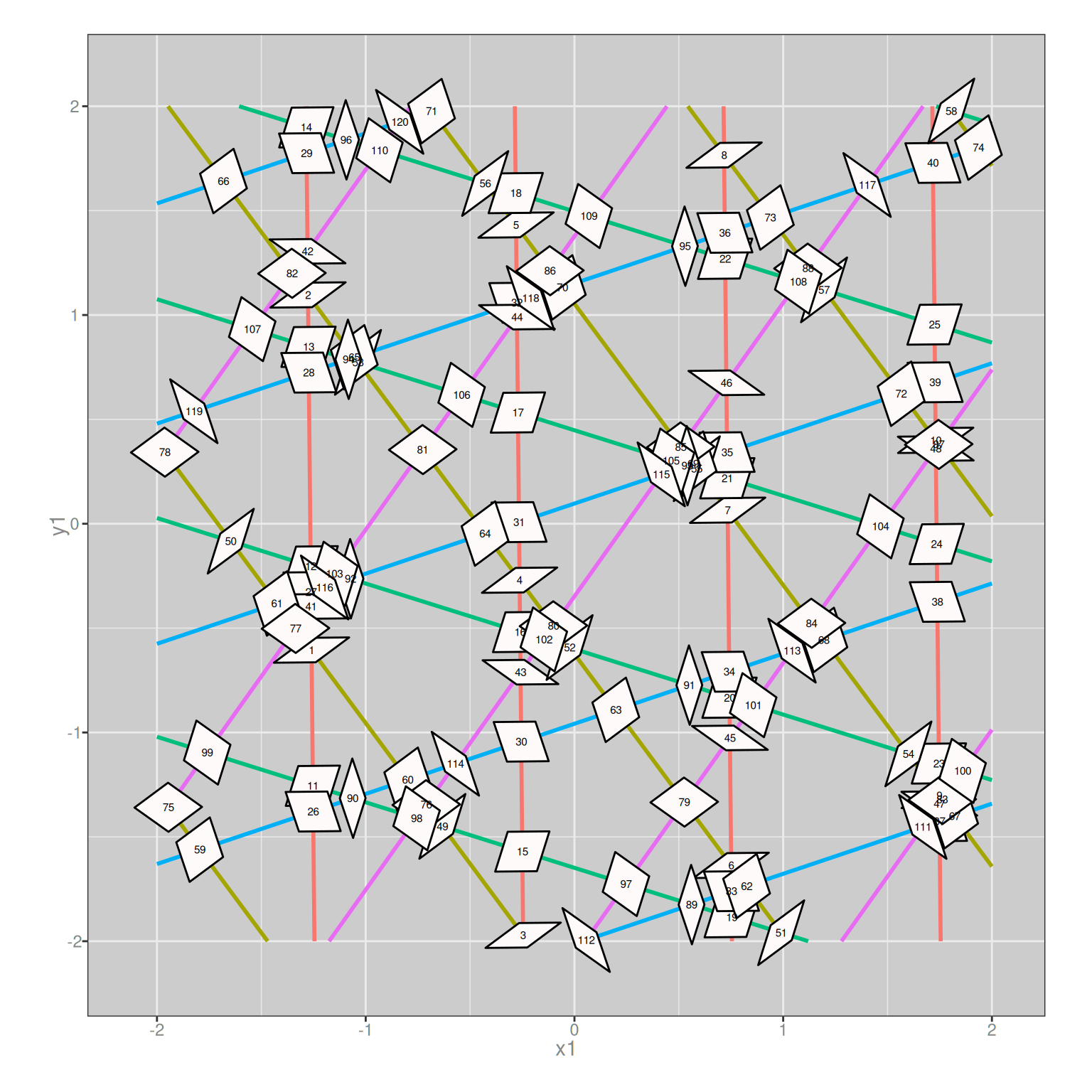
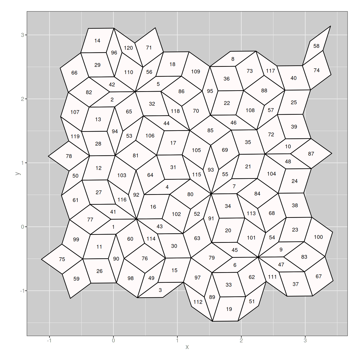
The plots below show what happens this time. On the left, you can see the grid lines as they are produced when n_families = 5, with the rhombus tiles placed in their original locations on top of grid intersections. On the right, you can see what the assembled tiling looks like:
This has some potential, but it could do with a splash of colour.
A convenient palette construction tool
This post is getting awfully long, so rather than come up with a new system for generating palettes I’ll reuse the linear cosine palette technique I wrote about in a previous post. We can use the cosine_palette() function to create a custom palette from a single seed value:
# Builds a random instance of Inigo Quilez's cosine-based colour palette
# (https://iquilezles.org/articles/palettes/): each RGB channel varies
# smoothly as `a + b * cos(2*pi*(c*t + d))` for t in [0, 1], where a, b, c,
# d are length-3 vectors. Returns a function of n (the number of colours
# needed) rather than a fixed palette, so that calling it again with a
# different n re-samples the same underlying curve.
cosine_palette <- function(seed = NULL) {
  if (!is.null(seed)) set.seed(seed)
  base <- colors(distinct = TRUE)
  function(n) {
    a <- c(0.5, 0.5, 0.5)
    b <- (sample(base, 1) |> col2rgb() |> as.vector()) / 255
    c <- (sample(base, 1) |> col2rgb() |> as.vector()) / 255
    d <- (sample(base, 1) |> col2rgb() |> as.vector()) / 255
    # evaluate the palette curve at n evenly-spaced points along [0, 1]
    pal <- vapply(
      seq(0, 1, length.out = n),
      function(t) a + b * cos(2 * pi * (c * t + d)),
      double(3)
    )
    # the cosine formula can occasionally push a channel outside [0, 1];
    # clip before converting to a valid hex colour
    pal[pal > 1] <- 1
    rgb(t(abs(pal)))
  }
}
This cosine_palette() tool is a function factory: it returns a function that takes an argument n and then returns a vector of n colours that can be used to provide whatever colouring we need for our de Bruijn tilings. In case you haven’t read the previous post, here’s a few examples of what smoothly varying cosine palettes look like:












For the de Bruijn tilings we’ll only ever need a small number of colours, but the capability exists for something much more continuous if that’s ever needed.
Building and plotting the tiling
Now all that remains to do is write some top-level functions to create plots. There two functions that do most of the orchestration work:
build_debruijn_tiling()builds the full data structure for a de Bruijn tiling, for user-specified choice ofn_families, apalettefunction, and an axisscale.plot_debruijn_tiling()takes the assembledtilingas input and creates the plot, after cropping it suitably so that the tiling completely fills a square plot area.
The one that you’d call, however, is this one:
random_debruijn_tiling()takes a user-specifiedseedas input (and optionally, anaxis_scaleparameter) and generates a randomly selected de Bruijn tiling.
Here’s the code for all three:
# Build the full data structure for one random de Bruijn tiling: draws random
# phase offsets, computes the grid-line intersections, turns each one into a
# rhombus, and glues all rhombi into a single assembled tiling. Returns a
# tidy data frame (one row per tile vertex) ready for ggplot2.
build_debruijn_tiling <- function(n_families, palette, scale) {

  # `scale` is the overall bounding box size; dividing by n_families keeps
  # the *density* of grid lines (and hence the number of tiles) roughly
  # comparable across different n_families, since more line families
  # means more lines crossing any given region. `tile_scale` separately
  # controls the physical size of each individual rhombus and is left
  # fixed at 1. build_tiling() has its own `scale` argument for this,
  # unused here, since build_rhombus() already bakes the size in
  x_scale <- scale / n_families
  y_scale <- scale / n_families
  tile_scale <- 1

  # The grid construction pipeline: random phases -> clipped grid lines ->
  # pairwise intersections of those lines (one per rhombus)
  offsets <- sample_offsets(n_families)
  lines <- build_grid_lines(x_scale, y_scale, offsets)
  inter <- find_intersections(lines)

  # Turn every intersection into its own independent rhombus (vertices +
  # metadata); build_rhombus()'s arguments are named to match
  # `intersections`'s columns, so pmap() can call it row-by-row directly
  rhombi_raw <- inter |>
    mutate(scale = tile_scale) |>
    pmap(build_rhombus)

  # Re-shape the list of individually-built rhombi into the two parallel
  # structures that compute_neighbours() and build_tiling() expect: a plain
  # list of vertex matrices, and a single properties tibble with one row
  # per tile (tagged with a matching `idx`, 1-based in list order)
  rhombi_tbl <- list(
    vertices = rhombi_raw |> map(\(r) r$vertices),
    properties = rhombi_raw |>
      imap_dfr(\(r, idx) r$properties, .id = "idx") |>
      mutate(idx = as.numeric(idx))
  )

  # Figure out which tiles are edge-to-edge neighbours, then glue them all
  # together into one consistent, gap-free assembly
  neighbours <- compute_neighbours(rhombi_tbl)
  placed <- build_tiling(rhombi_tbl, neighbours)

  # Colour each tile by its (rounded) smallest internal angle, so each
  # distinct rhombus shape gets its own colour; this mirrors the Python
  # original, but is not the only way to decide on tile colouring
  bucketed <- round(rhombi_tbl$properties$tile_acute, 4)
  unique_angles <- sort(unique(bucketed))
  tile_palette <- palette(length(unique_angles))
  tile_colour <- tile_palette[match(bucketed, unique_angles)]

  # A handful of rhombi right at the box edge can end up with no shared-line
  # neighbours and are never reached by the BFS; drop those rather than erroring
  reached <- !map_lgl(placed, is.null)
  if (!all(reached)) {
    message(
      sum(!reached),
      " isolated edge tile(s) dropped from the assembled tiling"
    )
  }

  # Flatten the list of per-tile vertex matrices into one tidy data frame,
  # one row per vertex, ready for plotting
  which(reached) |>
    map_dfr(\(idx) {
      r <- placed[[idx]]
      tibble(
        tile_id = idx,
        vertex = 1:4,
        x = r[, 1],
        y = r[, 2],
        colour = tile_colour[idx]
      )
    })
}
# Render an assembled tiling with each rhombus shaded according to its shape
# (based on smallest internal angle)
plot_debruijn_tiling <- function(tiling) {
# Horizontal range spanned by the tiling
x_min <- min(tiling$x)
x_max <- max(tiling$x)
# Vertical range spanned by the tiling
y_min <- min(tiling$y)
y_max <- max(tiling$y)
# Spans along both dimension
x_extent <- x_max - x_min
y_extent <- y_max - y_min
# Decide on a common width and cropping for the plot
extent <- min(c(x_extent, y_extent))
crop <- extent * .2
# Axis limits
xlim <- c(x_min + crop, x_min + extent - crop)
ylim <- c(y_min + crop, y_min + extent - crop)
# Build and return the plot
tiling |>
ggplot(aes(x = x, y = y, group = tile_id, fill = colour)) +
geom_polygon(colour = "black", linewidth = 0.15) +
scale_fill_identity() +
scale_x_continuous(expand = c(0, 0)) +
scale_y_continuous(expand = c(0, 0)) +
coord_equal(xlim = xlim, ylim = ylim) +
theme_void()
}random_debruijn_tiling <- function(seed, axis_scale = 100) {
set.seed(seed)
# High level parameters
n_families <- sample(5:10, size = 1)
palette <- cosine_palette(seed)
# Generate the tiling data structure
tiling <- build_debruijn_tiling(
n_families = n_families,
palette = palette,
scale = axis_scale
)
# Return the corresponding ggplot2 object
plot_debruijn_tiling(tiling)
}Example plots
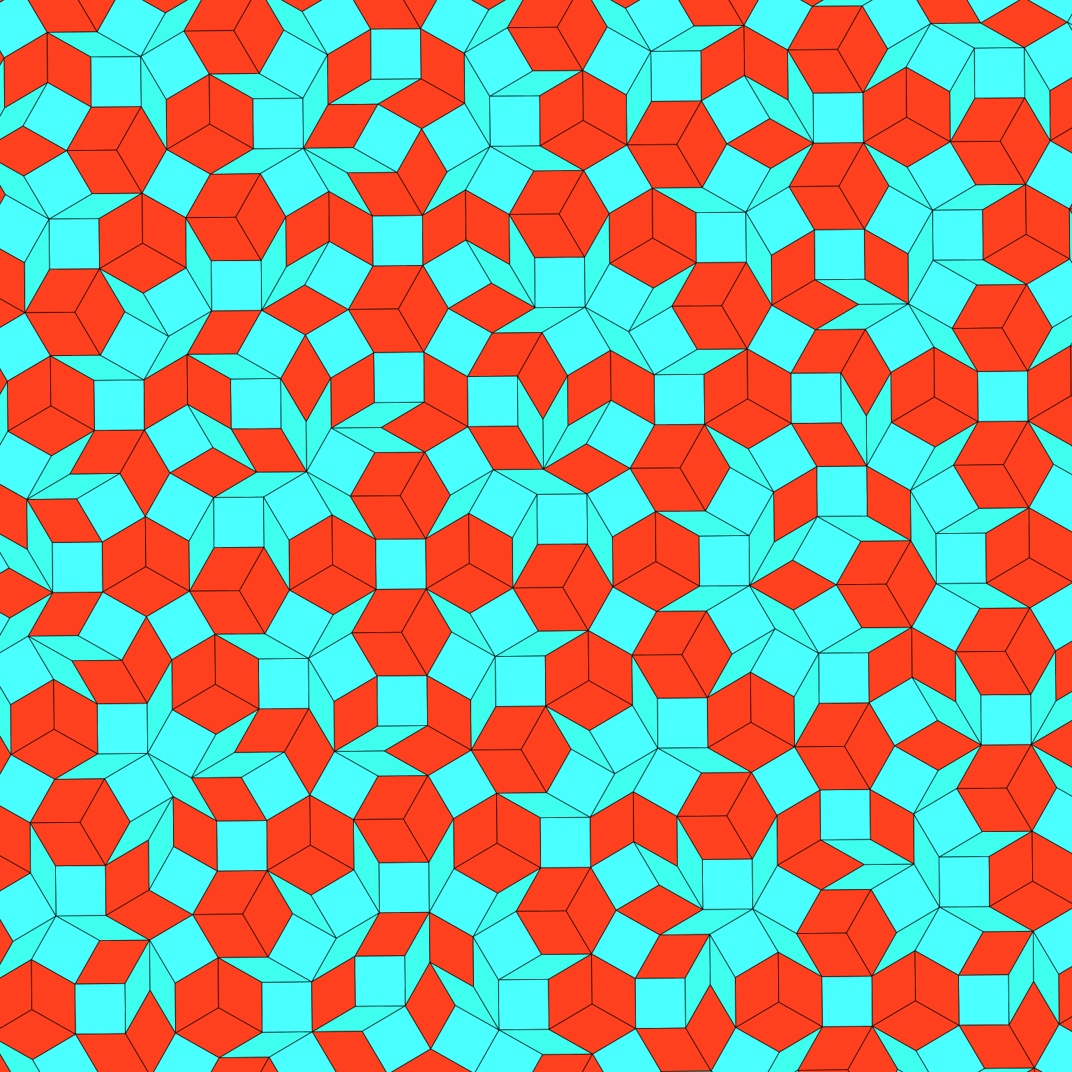
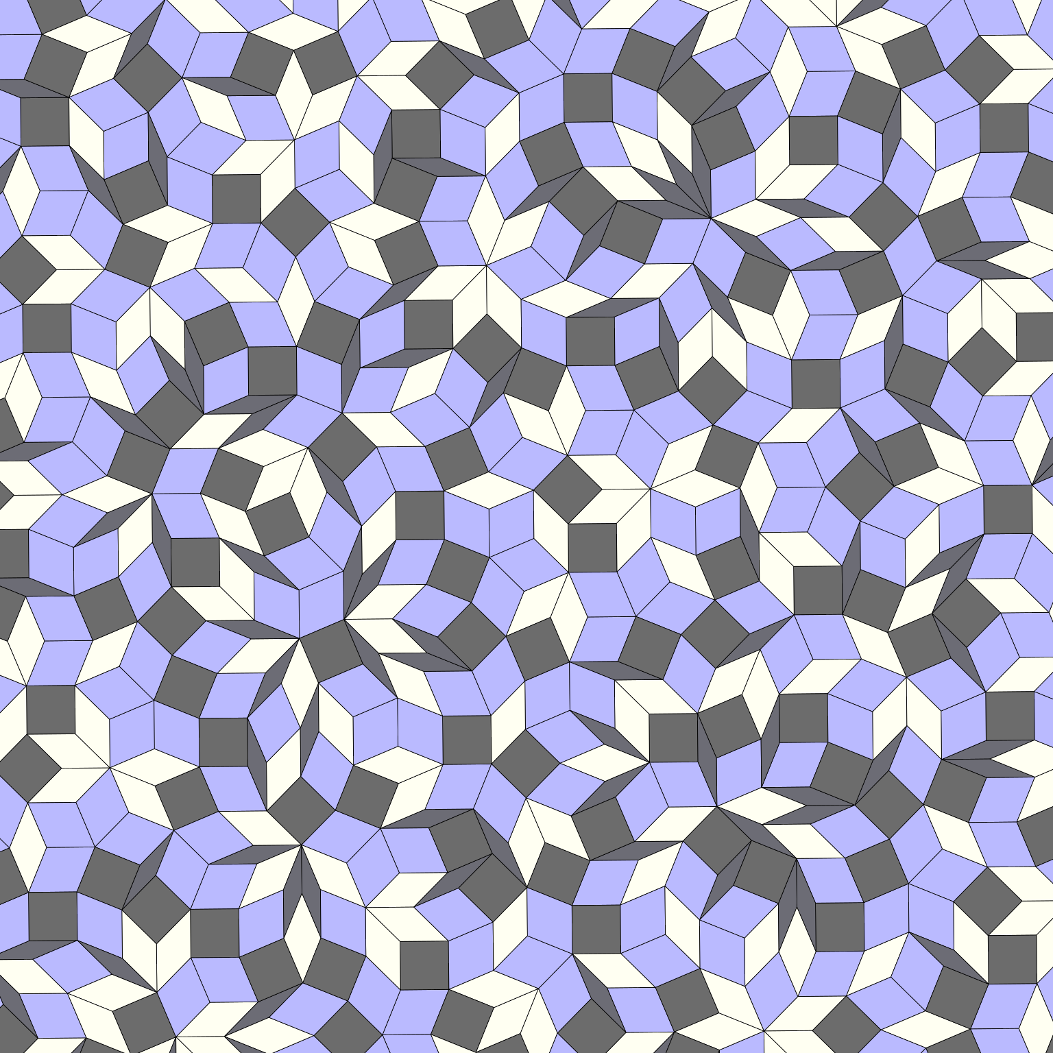
Now that we have the entire art pipeline out, let’s see what it can do. Here are three random de Bruijn tilings produced by changing the seed:
random_debruijn_tiling(seed = 1, axis_scale = 25)
random_debruijn_tiling(seed = 2, axis_scale = 25)
random_debruijn_tiling(seed = 3, axis_scale = 25)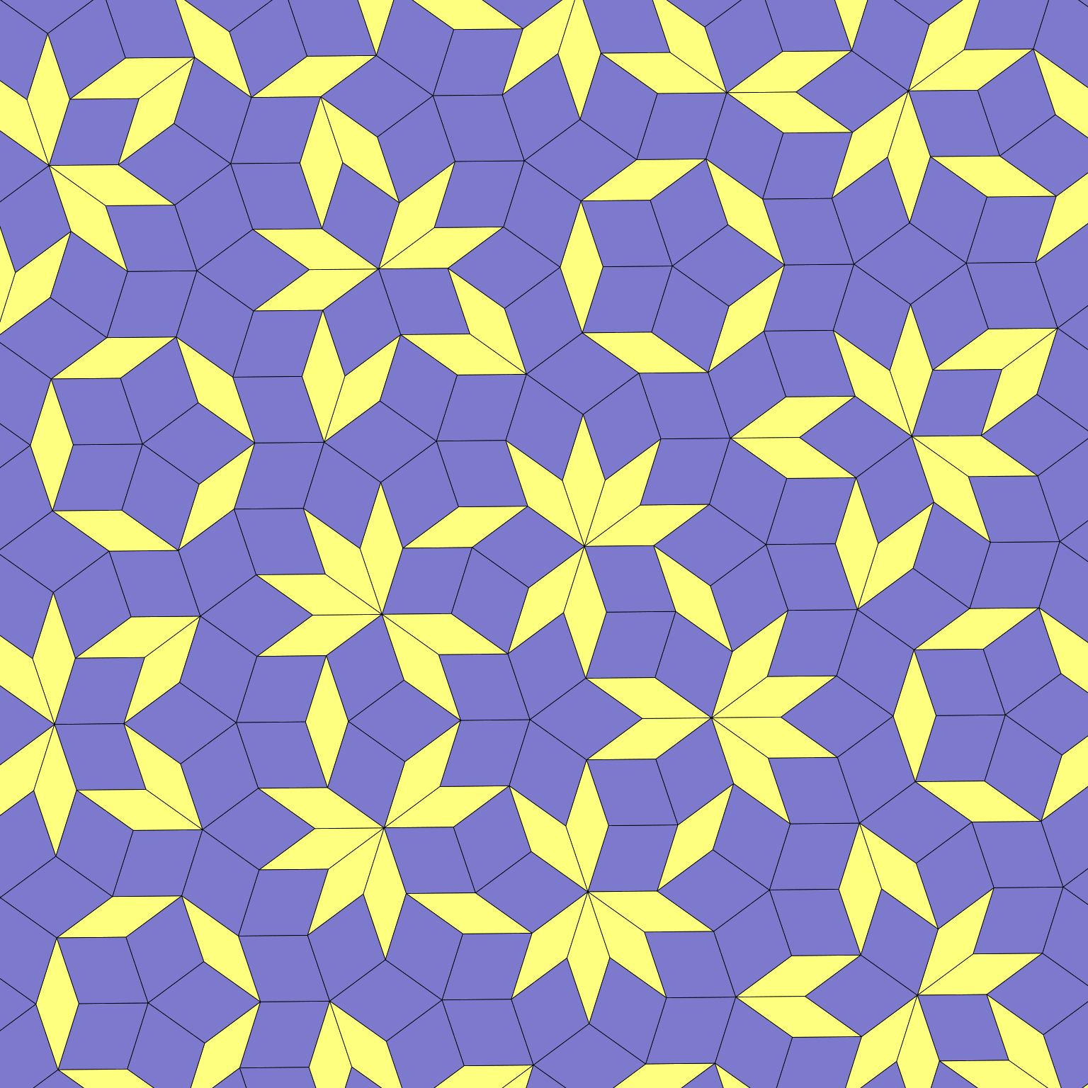
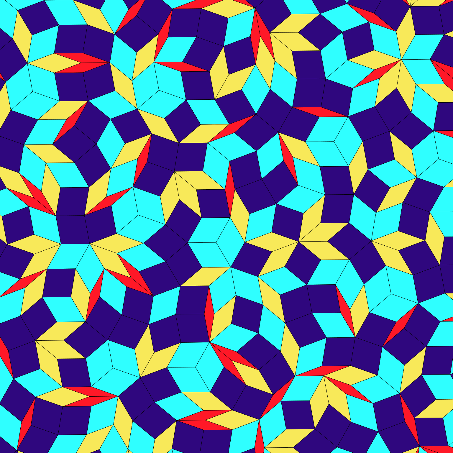
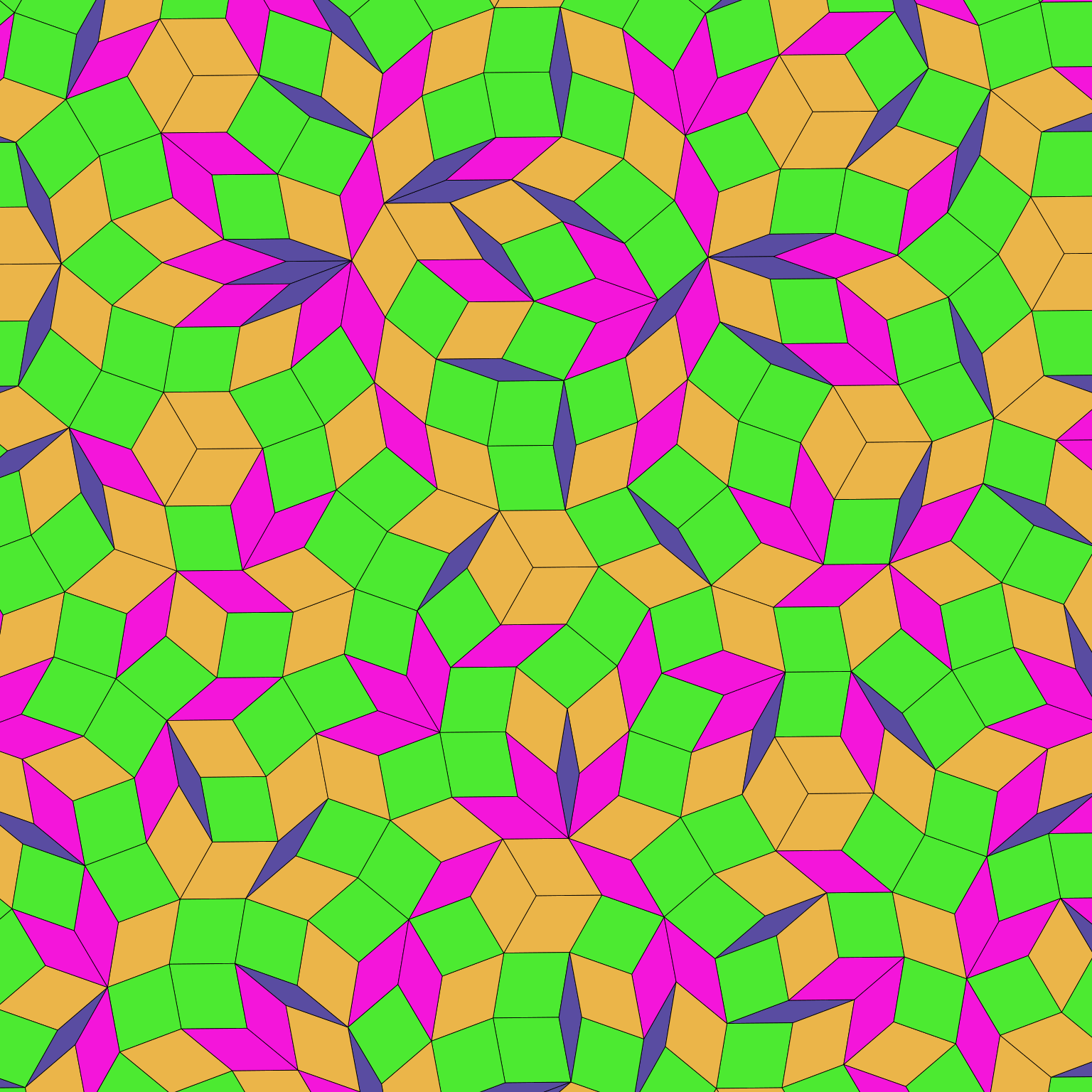
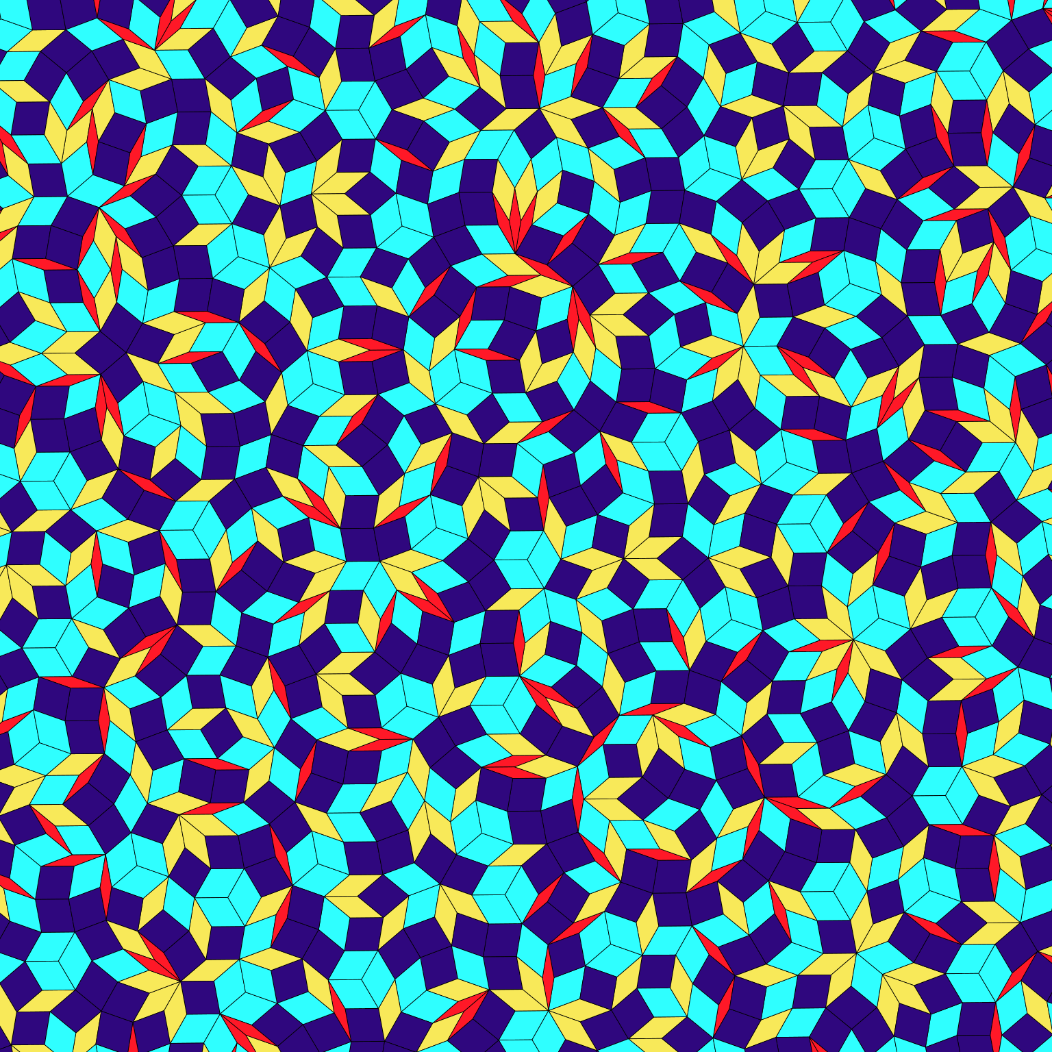
These are the same three tilings, but the plot is now zoomed out somewhat so you can see what it looks like on a different scale:
random_debruijn_tiling(seed = 1, axis_scale = 50)
random_debruijn_tiling(seed = 2, axis_scale = 50)
random_debruijn_tiling(seed = 3, axis_scale = 50)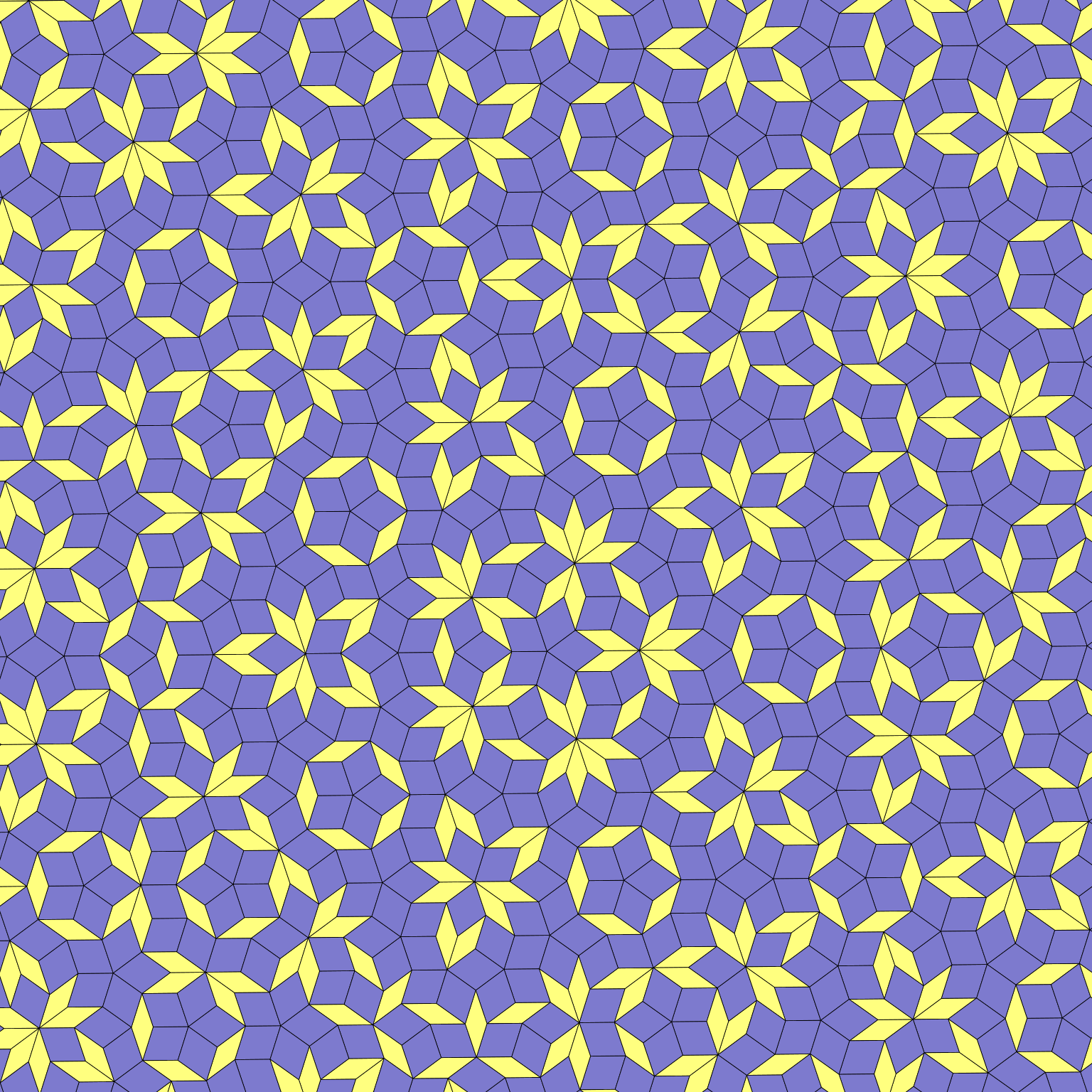
Epilogue
One of the peculiar things about this post, from my perspective, is that nothing I’ve done here goes very far beyond the code that was already available from other sources. It is not much more than a port of the Python library that I mentioned at the start of the post, and does nothing except re-implement the base R version that Claude wrote for me originally. But there is something fundamentally different about this version: it is mine. I wrote this code. I taught myself how to build de Bruijn tilings properly, and having done so I understand what the script does at a deep level. In the process I corrected some subtle bugs in the base R version, wrote explanatory notes that make sense to me, and the result of this effort is that I feel a stronger sense of artistic ownership of the outputs. Every image in this post comes from my code, not someone else’s.
To my mind, this matters. The images that appeared in the ntile post don’t feel like my art: I didn’t make them, and I don’t feel any sense of accomplishment at their creation. The images in this post are different. They are my work in a much deeper sense, and while I might not have gone very far along this particular artistic path, this art is mine. Art is not about the output, not really. The process matters, the artistic story behind it matters, and even in an art form as mechanistic as generative art there is no clean separation between art and artist. If you break that link you don’t have art anymore, all you have is a pretty picture.
References
- The original article by N. G. de Bruijn.
- The samacqua/tilings Python library by Sam Acquaviva.
- A discussion of de Bruijn tilings by Adam Ponting, in turn based on notes here.
Source code
If you would like to play around with these tilings yourself, the script below contains the source code for all functions that this post uses to build them.
# Packages
library(ggplot2)
library(tibble)
library(purrr)
library(tidyr)
library(dplyr)
# Every intersection of two grid lines becomes a rhombus, in the usual
# "dual" construction for these grid methods: the rhombus edges run
# perpendicular to the two line directions that cross at this point, and
# its two pairs of opposite edges have length `2 * scale`.
build_rhombus <- function(x_mid,
y_mid,
angle_1,
angle_2,
offset_1 = NA_real_,
offset_2 = NA_real_,
family_1 = NA_real_,
family_2 = NA_real_,
line_1 = NA_real_,
line_2 = NA_real_,
scale = 1) {
# Rhombus edge directions are rotated 90 degrees from the line angles;
# this ensures that rhombi that sit on the same line will have matching
# faces, and can be tiled next to one another without gaps when the
# tiling is assembled
rh_angle_1 <- angle_1 + pi / 2
rh_angle_2 <- angle_2 + pi / 2
# These are unit vectors pointing along the two pairs of edges
d1 <- c(-sin(rh_angle_1), cos(rh_angle_1))
d2 <- c(-sin(rh_angle_2), cos(rh_angle_2))
# Centroid coordinates as a named vector; names become the column names
# for the vertices matrix, and later become column names for the data
# frame
centre <- c(x = x_mid, y = y_mid)
# The four corners, reached from the centre by moving +/- scale along
# each of the two edge directions in turn; it is convenient to represent
# vertices as a matrix rather than a data frame, even though plotting is
# easier in the latter format.
vertices <- rbind(
centre + scale * d1 + scale * d2,
centre - scale * d1 + scale * d2,
centre - scale * d1 - scale * d2,
centre + scale * d1 - scale * d2
)
# The angle *between* the two grid-line directions determines the shape
# of the rhombus (a 72-degree gap between line families gives "thin"
# Penrose rhombi, a 36-degree gap gives "fat" ones, etc). Reducing this
# angle to its smallest equivalent (the acute angle, <= pi/2) gives a
# single number that identifies the tile's shape regardless of its
# orientation: it's not strictly needed to construct the tiling, but gets
# used later to decide the fill colour of a tile
diff <- abs((rh_angle_2 - rh_angle_1) %% (2 * pi))
if (diff > pi) diff <- 2 * pi - diff
tile_acute <- if (diff > pi / 2) pi - diff else diff
# Return the built rhombus as a list containing a matrix of vertices,
# plus a one-row tibble of metadata: the acute angle (for colouring)
# and, crucially, *which* two grid lines (family + line index) this
# tile sits on. Keeping track of this is critical for the tiling process,
# since compute_neighbours() and build_tiling() later match tiles up by
# looking for shared (family, line) pairs
list(
vertices = vertices,
properties = tibble(
tile_acute = tile_acute,
x_mid = x_mid,
y_mid = y_mid,
angle_1 = angle_1,
angle_2 = angle_2,
offset_1 = offset_1,
offset_2 = offset_2,
family_1 = family_1,
family_2 = family_2,
line_1 = line_1,
line_2 = line_2
)
)
}
# There's no probabilistic component to setting the angles that define
# the line families; only to the horizontal offsets that displace them.
# The default value to `angle_offset` is deliberately slightly non-zero,
# which means that angles are not *strictly* defined relative to north,
# but are ever so slightly rotated. This is purely a numerical convenience,
# to avoid issues that pop up with vertical lines (infinite slope)
build_families <- function(n_families,
offsets = NULL,
angle_offset = 0.01,
seed = NULL) {
# if the line family offsets aren't set, generate them randomly
if (is.null(offsets)) offsets <- sample_offsets(n_families, seed = seed)
# return a tibble with summary information for each line family
tibble(
family = seq_len(n_families),
offset = offsets,
angle = (family - 1) * pi / n_families + angle_offset
)
}
# Each of the line families is offset horizontally from the origin by a phase
# These phases are what make the resulting tiling look "random"
sample_offsets <- function(n_families, eps = 1e-6, seed = NULL) {
if (!is.null(seed)) set.seed(seed)
offsets <- runif(n_families)
repeat {
bad <- outer(offsets, offsets, function(a, b) abs(a - b) < eps) |
outer(offsets, offsets, function(a, b) abs(a + b - 1) < eps)
diag(bad) <- FALSE
if (!any(bad)) break
idx <- which(rowSums(bad) > 0)
offsets[idx] <- runif(length(idx))
}
offsets
}
# Handy little infix operator to check if a scalar value falls within the
# range specified by a length-2 vector
`%within%` <- function(value, range) range[1] <= value & value <= range[2]
# Build the families of parallel lines, and populate each family with a
# sufficient number of lines to fill the bounding box (defined by the
# x_scale and y_scale parameters). Returns a data frame with one row for
# each line that passes through the bounding box, with coordinates and
# other useful information.
build_grid_lines <- function(x_scale,
y_scale,
offsets,
eps = 1e-6) {
# Set up the line families
n_families <- length(offsets)
families <- build_families(n_families, offsets)
# Define the bounding box; keep this internal because it's not really a
# plot limit; it behaves like a plot limit for the purposes of this
# function, but when the final tiling gets assembled the rhombi get moved
# around, so the final plot limits are different
xlim <- c(-x_scale, x_scale)
ylim <- c(-y_scale, y_scale)
# For each family, work out which integer `line` values could possibly
# intersect the box at all, so later steps don't waste time clipping
# lines that are nowhere near it. `corner_k` evaluates the line equation
# `x*cos(angle) + y*sin(angle) + offset` at each of the box's 4 corners.
# The resulting range of `line` must cover every integer between the
# smallest and largest corner value (with a 1-unit pad on each side, to
# be safe about rounding) for the family's lines to span the box
line_cases <- families |>
cross_join(expand_grid(xlim, ylim)) |>
mutate(corner_k = xlim * cos(angle) + ylim * sin(angle) + offset) |>
reframe(
.by = family,
across(c(offset, angle), first),
line = seq(
from = floor(min(corner_k)) - 1,
to = ceiling(max(corner_k)) + 1
)
)
# Function to clip one specific line (one `family`/`line` combination)
# to the bounding box. A line can leave the box through a horizontal edge
# (at y = ylim) or a vertical edge (at x = xlim); this solves for both and
# keeps only the crossing points that are actually within the box
# (`x_ok`/`y_ok`), then de-duplicates in case a line passes exactly
# through a corner. Near-horizontal/near-vertical lines need the
# opposite equation (division by a near-zero cos/sin), which is why both
# cases are computed and only the valid one(s) kept via `eps`.
build_grid_line <- function(family, offset, angle, line) {
points <- bind_rows(
tibble(
y = ylim,
x = (line - offset - y * sin(angle)) / cos(angle),
x_ok = x %within% xlim,
y_ok = abs(sin(angle)) > eps
),
tibble(
x = xlim,
y = (line - offset - x * cos(angle)) / sin(angle),
y_ok = y %within% ylim,
x_ok = abs(cos(angle)) > eps
)
)
points <- points |>
filter(x_ok & y_ok) |>
distinct()
# A line that misses the box entirely contributes no segment. This
# isn't expected to happen normally, but retained just in case
if (nrow(points) == 0) {
return(tibble(
family = numeric(0),
line = numeric(0),
angle = numeric(0),
offset = numeric(0),
x1 = numeric(0),
y1 = numeric(0),
x2 = numeric(0),
y2 = numeric(0)
))
}
tibble(
family = family,
line = line,
angle = angle,
offset = offset,
x1 = points$x[1],
y1 = points$y[1],
x2 = points$x[2],
y2 = points$y[2]
)
}
# Clip every candidate line in every family, and return a tibble
line_cases |> pmap_dfr(build_grid_line)
}
# Find every point where a line from one family crosses a line from
# another family, within the bounding box. Lines in the same family
# are parallel, so the search is performed across pairs of lines that
# belong to different families.
find_intersections <- function(lines,
x_scale = NULL,
y_scale = NULL,
eps = 1e-10) {
# Detect the box scale from the lines if the user doesn't specify
if (is.null(x_scale)) x_scale <- max(abs(c(lines$x1, lines$x2)))
if (is.null(y_scale)) y_scale <- max(abs(c(lines$y1, lines$y2)))
# As before: keep this internal because it's not really a plot limit
xlim <- c(-x_scale, x_scale)
ylim <- c(-y_scale, y_scale)
# Find all unique pairs of line families: the base R combn() function
# is more efficient in general but expand_grid() then filter() is
# perfectly fine here
family <- sort(unique(lines$family))
family_pairs <- expand_grid(family_1 = family, family_2 = family) |>
filter(family_2 > family_1)
# Helper function used to detect all the intersections between two
# line families that fall inside the plotting area
find_family_intersections <- function(family_1, family_2) {
# Empty tibble to return if there is no intersection
null_intersection <- tibble(
x = numeric(0),
y = numeric(0),
angle_1 = numeric(0),
angle_2 = numeric(0),
offset_1 = numeric(0),
offset_2 = numeric(0),
family_1 = numeric(0),
family_2 = numeric(0),
line_1 = numeric(0),
line_2 = numeric(0)
)
# Sets of lines associated with each of the two families
line_set_1 <- lines |> filter(family == family_1)
line_set_2 <- lines |> filter(family == family_2)
# The angles specifying the two line families
angle_1 <- line_set_1$angle[1]
angle_2 <- line_set_2$angle[1]
# The offsets associated with the two line families
offset_1 <- line_set_1$offset[1]
offset_2 <- line_set_2$offset[1]
# Take sin and cosine of both angles
cos_a1 <- cos(angle_1)
sin_a1 <- sin(angle_1)
cos_a2 <- cos(angle_2)
sin_a2 <- sin(angle_2)
# Return an empty tibble if the determinant is too low. When
# det = 0 the lines are exactly parallel and no intersection
# exists. A threshold is applied to avoid numerical issues
# that arise with nearly-parallel lines
det <- cos_a1 * sin_a2 - cos_a2 * sin_a1
if (abs(det) < eps) return(null_intersection)
# Determine an "adjusted" coordinate for each line, after taking
# family-specific offset values into account; then compute the x
# and y values at which the intersection occurs; retaining only
# those intersections that remain within the plot limits
grid <- expand_grid(
line_1 = line_set_1$line,
line_2 = line_set_2$line
) |>
mutate(
line_coord_1 = line_1 - offset_1,
line_coord_2 = line_2 - offset_2,
x = (line_coord_1 * sin_a2 - line_coord_2 * sin_a1) / det,
y = (line_coord_2 * cos_a1 - line_coord_1 * cos_a2) / det,
keep = (x %within% xlim) & (y %within% ylim)
) |>
filter(keep)
# If none of the pairs are retained return an empty tibble
if (nrow(grid) == 0) return(null_intersection)
# Return a tibble containing the retained intersections
grid |>
transmute(
x = x,
y = y,
angle_1 = angle_1,
angle_2 = angle_2,
offset_1 = offset_1,
offset_2 = offset_2,
family_1 = family_1,
family_2 = family_2,
line_1 = line_1,
line_2 = line_2
)
}
family_pairs |> pmap_dfr(find_family_intersections)
}
# Find consecutive pairs for every grid line, and returns them as a tidy
# edge list (idx, neighbour), with each pair listed in both directions so
# the breadth-first search that comes later in build_tiling() can look up
# neighbours from either side.
compute_neighbours <- function(rhombi_tbl) {
props <- rhombi_tbl$properties
# Pivot from one-row-per-tile to one-row-per-(tile, side): every tile
# contributes two rows, one for each of the two grid lines it sits on.
# In this context bind_rows() is simpler than using pivot_longer()
sides <- bind_rows(
props |> select(
idx, family = family_1, line = line_1,
angle = angle_1, x_mid, y_mid
),
props |> select(
idx, family = family_2, line = line_2,
angle = angle_2, x_mid, y_mid
)
)
edges <- sides |>
# Tiles strung along a grid line can be fully ordered by their position
# along the line: `proj` takes the centre of the tile and projects it
# onto the direction perpendicular to the line, and increases monotonically
# as you move along the line
mutate(proj = -sin(angle) * x_mid + cos(angle) * y_mid) |>
# Sorting tiles within each (family, line) group by the projected position,
# ensures that tiles adjacent in the sorted order are exactly the tiles
# adjacent in physical space along the line
arrange(family, line, proj) |>
# Pair each tile with the very next one in sorted order, within its
# group. These are edge-sharing neighbour pairs.
mutate(neighbour = lead(idx), .by = c(family, line)) |>
filter(!is.na(neighbour)) |>
select(idx, neighbour)
# Each pair was only recorded in one direction (idx -> neighbour); add
# the mirror-image rows so the relation is symmetric
edges_reversed <- edges |> rename(idx = neighbour, neighbour = idx)
bind_rows(edges, edges_reversed) |> distinct()
}
# Centre a set of vertices on the origin
centre_vertices <- function(vertices, scale = 1) {
sweep(vertices, 2, colMeans(vertices)) * scale
}
# Project every row of `vertices` (a matrix of x,y points) onto a direction
# vector; this gives, for each vertex, its signed distance along `direction`
# (vertices further "ahead" in that direction get larger values). If we set
# `farthest = TRUE` the function picks out the vertex (or vertices, because
# for our rhombi there will always be two of these) with the largest projection
# along this direction. If we set `farthest = FALSE` it does the opposite,
# and returns the vertices with the smallest projection
extreme_vertices <- function(vertices, direction, farthest = TRUE) {
proj <- as.numeric(vertices %*% direction)
extreme <- if (farthest) max(proj) else min(proj)
vertices[abs(proj - extreme) < 1e-8, , drop = FALSE]
}
# Slot the neighbour tile ("nbr") into place immediately next to the current
# tile ("cur"), using only the information available at placement time. That
# includes the properties for both tiles (`props_cur` and `props_nbr`), as
# well as the already-placed location of the current tile (`placed_cur`) and
# the "centred" location for the neighbour tile (`centred_nbr`; i.e., the
# neighbour tile centred on the origin).
shift_neighbour <- function(props_cur, props_nbr, placed_cur, centred_nbr) {
# Each tile sits on exactly two grid lines (its two "sides"); a pair of
# neighbouring tiles will have one of these in common. Find the shared
# (family, line) pair and pull out the angle associated with that family.
# This is the direction of the grid line that the shared edge lies on.
sides_cur <- tibble(
family = c(props_cur$family_1, props_cur$family_2),
line = c(props_cur$line_1, props_cur$line_2),
angle = c(props_cur$angle_1, props_cur$angle_2)
)
sides_nbr <- tibble(
family = c(props_nbr$family_1, props_nbr$family_2),
line = c(props_nbr$line_1, props_nbr$line_2)
)
shared_angle <- sides_cur |>
semi_join(sides_nbr, by = c("family", "line")) |>
slice(1) |>
pull(angle)
# Direction vector `d` that points along the shared grid line
d <- c(-sin(shared_angle), cos(shared_angle))
# Decide whether the current tile was originally projected farther
# along direction `d` (i.e., `sgn > 0`) than the neighbouring tile,
# or whether it was projected less far along that direction
centre_cur <- c(props_cur$x_mid, props_cur$y_mid)
centre_nbr <- c(props_nbr$x_mid, props_nbr$y_mid)
sgn <- sign(sum((centre_nbr - centre_cur) * d))
if (sgn == 0) sgn <- 1
# Use extreme_vertices() to detect the "trailing" edge of the already-placed
# current tile, and the "leading" edge of the to-be-placed neighbouring tile.
# For our rhombi, which always have edges that are perpendicular to the
# relevant direction vector `d`, this will return two points, not one.
trailing_cur <- extreme_vertices(placed_cur, d, farthest = sgn > 0)
leading_nbr <- extreme_vertices(centred_nbr, d, farthest = sgn < 0)
# Calculate the shift needed to slide the neighbour tile so that the
# midpoint of its "leading" edge lands exactly on the midpoint of the
# current tile's "trailing" edge, thereby glueing the two edges together.
shift_nbr <- colMeans(trailing_cur) - colMeans(leading_nbr)
shift_nbr
}
# Assemble the complete tiling using breadth-first search
build_tiling <- function(rhombi_tbl, neighbours) {
# Pull the key information out of the rhombus list
vertices <- rhombi_tbl$vertices
props <- rhombi_tbl$properties
n <- nrow(props)
# Take each tile's vertex matrix and re-centre it on the origin by
# subtracting the column means (i.e. the centroid)
centred <- map(vertices, centre_vertices)
# `neighbours` is an edge list (idx, neighbour); split() turns it into a
# lookup table keyed by tile index, so neighbours_of(i) returns the
# vector of tile indices adjacent to tile i. split()'s keys become
# character strings, hence the as.character() when looking one up
adjacency <- split(neighbours$neighbour, neighbours$idx)
neighbours_of <- function(i) adjacency[[as.character(i)]]
# Define a seed tile from which to start the tiling
seed <- 1
# Define a `placed` list that will hold the final tiled locations of each
# of the rhombi. Initially it contains only the seed tile, in centred
# coordinates
placed <- vector("list", n)
placed[[seed]] <- centred[[seed]]
# The `seen` vector exists to keep track of which tiles have already been
# placed: an already-placed tile does not need to be moved again, even if
# it is a neighbour of the tile currently at the head of the queue
seen <- rep(FALSE, n)
seen[seed] <- TRUE
# Set up for the search: `queue` holds the tiles waiting to have their
# neighbours placed; `head` specifies the position within the queue that
# we are currently looking at
queue <- seed
head <- 1
# Breadth-first search; terminates when there is no new item at the "head"
# of the search queue. In this context the "head" is the current position
# in the queue, but the queue can grow by multiple elements in each cycle
# because one "current" tile might be used to connect more than one new
# "neighbour" tiles.
while (head <= length(queue)) {
# Read the current tile by inspecting the "head" of the queue, then
# advance the head location forward by 1 in anticipation of the next
# cycle
idx_cur <- queue[head]
head <- head + 1
# Place every neighbour of the current tile
for (idx_nbr in neighbours_of(idx_cur)) {
# If we've already seen the neighbour, skip it and move on
if (seen[idx_nbr]) next
# Rhombus vertices as they are currently known: the current tile
# has already been placed, but the neighbour is only centred
placed_cur <- placed[[idx_cur]]
centred_nbr <- centred[[idx_nbr]]
# Rhombus properties for both tiles
props_cur <- slice(props, idx_cur)
props_nbr <- slice(props, idx_nbr)
# Compute the shift required to move the centred neighbour tile
# into its placed location in the tiling
shift_nbr <- shift_neighbour(props_cur, props_nbr, placed_cur, centred_nbr)
# Move the neighbour tile into its placed location
placed[[idx_nbr]] <- sweep(centred[[idx_nbr]], 2, shift_nbr, "+")
# Note that the neighbour
seen[idx_nbr] <- TRUE
queue <- c(queue, idx_nbr)
}
}
# Return the list of placed vertex matrices, all expressed in the same
# edge-matched co-ordinate system. If a tile is never reached (which can
# happen if it has no neighbours due to how the grid lines crossed the
# bounding box earlier) it is left as a NULL entry in the list
placed
}
# Builds a random instance of Inigo Quilez's cosine-based colour palette
# (https://iquilezles.org/articles/palettes/): each RGB channel varies
# smoothly as `a + b * cos(2*pi*(c*t + d))` for t in [0, 1], where a, b, c,
# d are length-3 vectors. Returns a function of n (the number of colours
# needed) rather than a fixed palette, so that calling it again with a
# different n re-samples the same underlying curve.
cosine_palette <- function(seed = NULL) {
if (!is.null(seed)) set.seed(seed)
base <- colors(distinct = TRUE)
function(n) {
a <- c(0.5, 0.5, 0.5)
b <- (sample(base, 1) |> col2rgb() |> as.vector()) / 255
c <- (sample(base, 1) |> col2rgb() |> as.vector()) / 255
d <- (sample(base, 1) |> col2rgb() |> as.vector()) / 255
# evaluate the palette curve at n evenly-spaced points along [0, 1]
pal <- vapply(
seq(0, 1, length.out = n),
function(t) a + b * cos(2 * pi * (c * t + d)),
double(3)
)
# the cosine formula can occasionally push a channel outside [0, 1];
# clip before converting to a valid hex colour
pal[pal > 1] <- 1
rgb(t(abs(pal)))
}
}
# Build the full data structure for one random de Bruijn tiling: draws random
# phase offsets, computes the grid-line intersections, turns each one into a
# rhombus, and glues all rhombi into a single assembled tiling. Returns a
# tidy data frame (one row per tile vertex) ready for ggplot2.
build_debruijn_tiling <- function(n_families, palette, scale) {
# `scale` is the overall bounding box size; dividing by n_families keeps
# the *density* of grid lines (and hence the number of tiles) roughly
# comparable across different n_families, since more line families
# means more lines crossing any given region. `tile_scale` separately
# controls the physical size of each individual rhombus and is left
# fixed at 1. build_tiling() has its own `scale` argument for this,
# unused here, since build_rhombus() already bakes the size in
x_scale <- scale / n_families
y_scale <- scale / n_families
tile_scale <- 1
# The grid construction pipeline: random phases -> clipped grid lines ->
# pairwise intersections of those lines (one per rhombus)
offsets <- sample_offsets(n_families)
lines <- build_grid_lines(x_scale, y_scale, offsets)
inter <- find_intersections(lines)
# Turn every intersection into its own independent rhombus (vertices +
# metadata); build_rhombus()'s arguments are named to match
# `intersections`'s columns, so pmap() can call it row-by-row directly
rhombi_raw <- inter |>
mutate(scale = tile_scale) |>
pmap(build_rhombus)
# Re-shape the list of individually-built rhombi into the two parallel
# structures that compute_neighbours() and build_tiling() expect: a plain
# list of vertex matrices, and a single properties tibble with one row
# per tile (tagged with a matching `idx`, 1-based in list order)
rhombi_tbl <- list(
vertices = rhombi_raw |> map(\(r) r$vertices),
properties = rhombi_raw |>
imap_dfr(\(r, idx) r$properties, .id = "idx") |>
mutate(idx = as.numeric(idx))
)
# Figure out which tiles are edge-to-edge neighbours, then glue them all
# together into one consistent, gap-free assembly
neighbours <- compute_neighbours(rhombi_tbl)
placed <- build_tiling(rhombi_tbl, neighbours)
# Colour each tile by its (rounded) smallest internal angle, so each
# distinct rhombus shape gets its own colour; this mirrors the Python
# original, but is not the only way to decide on tile colouring
bucketed <- round(rhombi_tbl$properties$tile_acute, 4)
unique_angles <- sort(unique(bucketed))
tile_palette <- palette(length(unique_angles))
tile_colour <- tile_palette[match(bucketed, unique_angles)]
# A handful of rhombi right at the box edge can end up with no shared-line
# neighbours and are never reached by the BFS; drop those rather than erroring
reached <- !map_lgl(placed, is.null)
if (!all(reached)) {
message(
sum(!reached),
" isolated edge tile(s) dropped from the assembled tiling"
)
}
# Flatten the list of per-tile vertex matrices into one tidy data frame,
# one row per vertex, ready for plotting
which(reached) |>
map_dfr(\(idx) {
r <- placed[[idx]]
tibble(
tile_id = idx,
vertex = 1:4,
x = r[, 1],
y = r[, 2],
colour = tile_colour[idx]
)
})
}
# Render an assembled tiling with each rhombus shaded according to its shape
# (based on smallest internal angle)
plot_debruijn_tiling <- function(tiling) {

  # Horizontal range spanned by the tiling
  x_min <- min(tiling$x)
  x_max <- max(tiling$x)

  # Vertical range spanned by the tiling
  y_min <- min(tiling$y)
  y_max <- max(tiling$y)

  # Spans along both dimension
  x_extent <- x_max - x_min
  y_extent <- y_max - y_min

  # Decide on a common width and cropping for the plot
  extent <- min(c(x_extent, y_extent))
  crop <- extent * .2

  # Axis limits
  xlim <- c(x_min + crop, x_min + extent - crop)
  ylim <- c(y_min + crop, y_min + extent - crop)

  # Build and return the plot
  tiling |>
    ggplot(aes(x = x, y = y, group = tile_id, fill = colour)) +
    geom_polygon(colour = "black", linewidth = 0.15) +
    scale_fill_identity() +
    scale_x_continuous(expand = c(0, 0)) +
    scale_y_continuous(expand = c(0, 0)) +
    coord_equal(xlim = xlim, ylim = ylim) +
    theme_void()
}
# Top-level assembly
random_debruijn_tiling <- function(seed, axis_scale = 100) {
  set.seed(seed)

  # High level parameters
  n_families <- sample(5:10, size = 1)
  palette <- cosine_palette(seed)

  # Generate the tiling data structure
  tiling <- build_debruijn_tiling(
    n_families = n_families,
    palette = palette,
    scale = axis_scale
  )

  # Return the corresponding ggplot2 object
  plot_debruijn_tiling(tiling)
}Footnotes
- Sorry, no, you don’t get credit for crafting the prompt. It is not even remotely the same thing as writing the code, or crafting a photograph. Please be serious. The LLM has done all the heavy lifting for you, and at best you can claim to have asked it to do your work for you.↩︎
- The last 18 months have been a horror show in this regard, thanks to the curse of long covid and the occasional relapses I’ve had even after I started to recover from it. I spend waaaaaay too much of my life bedridden now, and it has not been good for me at all. I work on it as best I can, but fitness is very much a “use it or lose it” thing.↩︎
- Note that “pedagogical purposes” doesn’t just mean “I added it so that the audience would understand”. It also includes the fact that I will need to remind myself how I wrote this code later on, and for that reason I thought it worthwhile to retain all the notes-to-self that I wrote when translating Claude’s base-R code into something I found easier to work with.↩︎
Reuse
Citation
BibTeX citation:
@online{navarro2026,
  author = {Navarro, Danielle},
  title = {Aperiodic Tilings with the de {Bruijn} Method},
  date = {2026-10-01},
  url = {https://blog.djnavarro.net/posts/2026-10-01_debruijn-tilings/},
  langid = {en}
}
For attribution, please cite this work as: Navarro, Danielle. 2026. “Aperiodic Tilings with the de Bruijn Method.” October 1. .

 点赞
点赞 收藏
收藏 点踩
点踩 分享
分享