Sketched Isotropic Gaussian Regularization (SIGReg) Explained

The paper “LeJEPA: Provable and Scalable Self-Supervised Learning Without the Heuristics”(Balestriero and LeCun 2025) proposed an interesting method of regularizing latent spaces that I thought I’d explore.

This is a regularization technique to make latent embeddings have isotropic Gaussian distribution - each dimension is encouraged to be uncorrelated and independent, and gaussian distributed. They argue that gaussian latent embeddings are optimal because they are unbiased and lower variance for downstream tasks.

They make latent embeddings have Gaussian distribution using one-dimensional tests of normality in random directions via characteristic functions.

One-Dimension

ECDF Tests

First the paper motivates determining how Gaussian a distribution is with its empirical (i.e. observed) cumulative distribution function (ecdf). Lets look at this in one-dimension.

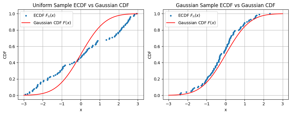
First we generate two “one sample” univariate datasets - one uniform and one standard gaussian. In this case the target distribution is the standard gaussian. Then we just compare the ecdfs with the theoretical gaussian cdf.

Code

Code

As you’d expect, in Figure 1 the ecdf of the uniform distribution sample deviates from the gaussian cdf having large gaps, but the gaussian sample does not.

We can quantify the “gap” or how close the empirical cdf is to the desired theoretical with the following formula,

where is the empirical cdf, is the theoretical cdf, and is a weighting function. With this is known the cramer-von-mise test statistic and is known as the anderson darling test statistic. We can compute this in scipy.

With some algebraic manipulation there are actually closed-form formulas for these test statistics. However, using the ecdf is still computationally expensive, and non-differentiable because it requires sorting the datasets. We calculate the cramer von mise and anderson darling test statistics below.

Code

As expected, the gaussian hypothesis is rejected for the uniform sample and not rejected for the gaussian sample.

Note: scipy.stats.anderson with dist set to “norm” tests for normality not standard normality and it does so by subtracting the sample mean and dividing by the sample standard deviation of your dataset.

Characteristic Functions

Although a distribution is uniquely defined by its cdf, it is also uniquely defined by its characteristic function. The characteristic function (CF) of a random variable is defined as,

where is the imaginary unit. For a sample we have empirical characteristic function (ECF),

Reminiscent of how the gap in cdf was defined, for CFs we can quantify the gap using,

which is known as the Epps-Pulley test. The weight function is typically which is also the theoretical CF for the Gaussian distribution.

The advantage of the Epps-Pulley test is that it’s differentiable and continuous i.e. if I move one data point a small amount the Epps-Pulley test statistic changes proportionally. In contrast, moving a data point would change the jumps in the ecdf which makes ecdf tests non-differentiable.

This integral can be estimated through the basic trapezoidal Riemann sum.

Code

The lower T statistic for the gaussian sample indicates less “gap”. I haven’t looked into the limiting distribution of the Epps-Pulley Test Statistic that would be used to calculate p-values.

We can also test the robustness to the number of divisions in the trapezoidal Riemann sum and see it converges quite quickly.

Code

Gradient Descent

Now we know how to quantify the gap between data and a target distribution with Epps-Pulley. Lets make a neural network output data that fits the desired target distribution. First lets send 1D data through a random, untrained neural network and check its output distribution.

Code

We can see the output isn’t very Gaussian. Now lets train the model using the Epps-Pulley Regularizer,

Code

Now we can see the trained model’s output is more Gaussian.

Multiple Dimensions

Multidimensional Gaussian Regularization

It’s not immediately clear how to apply this in higher dimensions without running into the curse of dimensionality. Naively approximating the integral in higher dimensions would require evaluating it at a number of points that scales exponentially with dimension. In the 1D example we used points. We want to avoid 2D requiring points, 3D requiring , and so on.

The paper’s idea is instead to sample directions in the -dimensional space, project the -dimensional points onto these directions, and then compute the corresponding univariate test statistics.

For a multivariate Gaussian random variable

any linear projection is also Gaussian. And when is a unit vector , the variance remains unchanged:

This means every projection of a standard isotropic Gaussian looks like:

The converse is what makes this useful: by the Cramér–Wold theorem, if every one-dimensional projection of a distribution is standard Gaussian, then the full multivariate distribution must itself be a standard(isotropic) multivariate Gaussian.

This gives us a scalable approximation strategy: instead of testing Gaussianity over the full -dimensional space, we test many random one-dimensional projections.

That’s the core idea behind SIGReg: approximate high-dimensional Gaussian regularization using randomized projections rather than exponentially expensive multidimensional integration.

Here I’ll demonstrate this in two dimensions. First, we’ll inspect scatter plots of 2D data, then choose a random direction on the 2D unit circle, project the points onto that direction, and examine the resulting histograms. The key observation is that these projections reduce the problem back to one dimension, where we can run the same Epps–Pulley test as before.

Code

SIGReg

SIGReg functions the same as above except takes the mean of slices. See the code block below which is similar to the code in the paper.

Code

Now lets make a network’s 10-dimensional output standard gaussian. We’ll plot a histogram in the direction of the first dimension, before and after training on the regularizer.

Code

Again, not very Gaussian. Lets train using SIGReg:

Code

And now after training, the output is more Gaussian. So adding this regularizer to your objective function encourages Gaussian latent embeddings.

In a future blog post, I’d like to train a small JEPA model using SIGReg as in “LeWorldModel: Stable End-to-End Joint-Embedding Predictive Architecture from Pixels”(Maes et al. 2026).

References

Balestriero, Randall, and Yann LeCun. 2025. LeJEPA: Provable and Scalable Self-Supervised Learning Without the Heuristics. arxiv.org/abs/2511.08544.

Maes, Lucas, Quentin Le Lidec, Damien Scieur, Yann LeCun, and Randall Balestriero. 2026. LeWorldModel: Stable End-to-End Joint-Embedding Predictive Architecture from Pixels. arxiv.org/abs/2603.19312.