Modelling variation in the METR Uplift Study

Disclaimer: Not associated with METR.

Summary

I reanalysed the METR uplift study under a meta-analytic model to estimate the range of plausible effects that we may see in repeated trials. If the average population effect varied as much as medical and economic Randomized Control Trials (RCTs), we would see a 95% credible interval of results from -55% to +193% even without study-specific effects. The mean population effect was between 10-20% with heavy tails. The probability of a slowdown is between 66% and 79%. The study was therefore compatible with both large speedups and slowdowns, even with no further AI progress.

We should be careful about drawing inferences on the sign or magnitude of AI-assistance when study variation is high, but this may explain the radically different effectiveness heard from self-reports. It would be good to find more ways of squeezing more information out of older data, since it is unlikely for us to gain more before the point of no return (if that isn't already passed).

AI speedups and slowdowns

The METR RCT remains the highest quality evidence that we have for developer productivity improvements using AI tools. The original METR uplift RCT was published in July 2025. It measured developer completion times from a selected set of issues from open source software projects. The headline result was developers were slower by 19% when using AI tools. This surprised many people, including expert forecasts, METR, and the developers themselves.

Given the widespread use of AI tools in software now, it is unlikely that these measurements will ever be repeated. Now, post Opus 4.8, Fable, Sol etc., there is a growing feeling that developers are sped up by at least 50% if not more. How can we know when we have definitively shifted in ability between models?

How to meta-analyse a single study

When we carry out an experiment, the end result is a measured effect from one variable to another. In the METR study, this effect is the logged ratio of the AI-assisted vs AI-disabled time-to-complete across all the projects. Let's call this .

There are many reasons that a single study may not reflect the real effect size. Studies can draw on different subjects, can measure the outcomes differently, and can use different techniques to elicit effects. Let's imagine that there really is one shared effect of AI-assistance on time-to-complete, and we can call this .

We can then build a generative model for what happens when a study is conducted. The measured effect size in a study , has both a inside-study error and a between-study error . You have the true population-size effect , the between-study effect and the residual error .

It's easy to see why this is beneficial when performing a traditional meta-analysis: you can weight every study by their inside-study error and combine them together to get a very confident result.

When only one study is present, the between-study effect is entirely defined by the prior. There's no way to get around this, since you don't have any data on the same topic to estimate from. In this circumstance, journal articles narratively discuss sources of study variation but often do not statistically correct for it. This assumes a very strong prior that the between-study variation is zero (or that the measured effect size is identical to the population effect size ). Experimentalists would be hard-pressed to assert that there is no effect caused by changes in study conditions, so here we can pick up accuracy left on the table.

We are left shrunk version of the effect size that is closer to the true study effect and wider confidence intervals which include the variation caused by differences in study conditions, as well as an estimate of the population effect .

Selecting priors on study variation

The problem with AI analysis is that there is very little evidence out there for these kind of effects. This leads to what some people have humorously called "reference-class tennis", where people use radically different priors based on incomparable sets of evidence. Empirical priors are typically drawn from evidence with a similar subject basis. Technology studies should have priors drawn from technology, economics from economics, medicine from medicine, etc. Instead, we can analyse under a variety of priors and study what the distribution of posteriors answers about the question, like in a multiverse study.

In the absence of any possible reference-class, we can try uninformative or weakly-informative priors. These priors are on the log scale of the predictor. At one extreme, there is the improper prior across the whole real number line: a of 0.1 is just as plausible as a of . This is very difficult to use because the estimator has to jump around between very different numbers. Instead, we can try a broad prior where and . This would imply a 95% credible interval of speed ups or slowdowns of ~16x. A 16x speedup or slowdown is at least physically possible if unrealistic (we would hopefully have noticed!), but from this we can understand how much of a difference the empirical priors have on the overall result.

For empirical priors, because we can't choose reference classes that are similar in subject, we instead try to select reference classes that are similar in statistical property. These should have similar levels of between-study variation. We should try to match:

• Meta-analyses with >5 measures
• Contain only randomised control trials
• Psychological or economic effects (as a proxy for similar variance in outcome)

You can find collated datasets for this purpose in BEAR.

I'm going to select from the Cochrane RCT database and the Askarov et al. 2023 collection of papers. There are 276 meta-analyses in the Cochrane data with more than 5 studies, although only 160 unique studies inside. For the Askarov dataset, there are only 6 meta-analyses and 33 unique studies. We're going to use these meta-analyses to estimate the amount of study variation, then apply these estimates as a prior to the METR uplift RCT. I use the hierarchical Bayesian model above to do this with the code from Zwet, Wiecek and Gelman (2025). I place uniform priors over parameters simply to identify their scale, but I choose to keep the estimate of the hyper-mean of to adjust different averages between RCTs.

Results

We start by estimating the average population effect and the study variation from the Cochrane and Askarov databases. The hypermean effect on or "average average population effect" in the Cochrane database is -0.22 and in the Askarov database it is -0.5. The number for Askarov is surprisingly extreme likely due to the small number of studies we have.

Similarly, the hypermean on or average study variation is 0.22 in the Cochrane database and 0.31 in the Askarov dataset for a ratio of 150%. This may represent genuine wider effect sizes in economics and we should consider this may also be true for effects caused by AI.

Raw info under the box

Mean of

SD of

(df)

Mean of log

SD of log

When estimating and for the METR study, I discard information about the average of since we don't know whether it should be a speedup or slowdown a priori, but I keep information about the variance and degrees of freedom of . We can go on then to estimate the five cases:

1) Uninformative prior

2 and 3) The Askarov (economic) data, with and without mean information

4 and 5) The Cochrane (medical) data, with and without mean information.

Inconclusive evidence of a slowdown

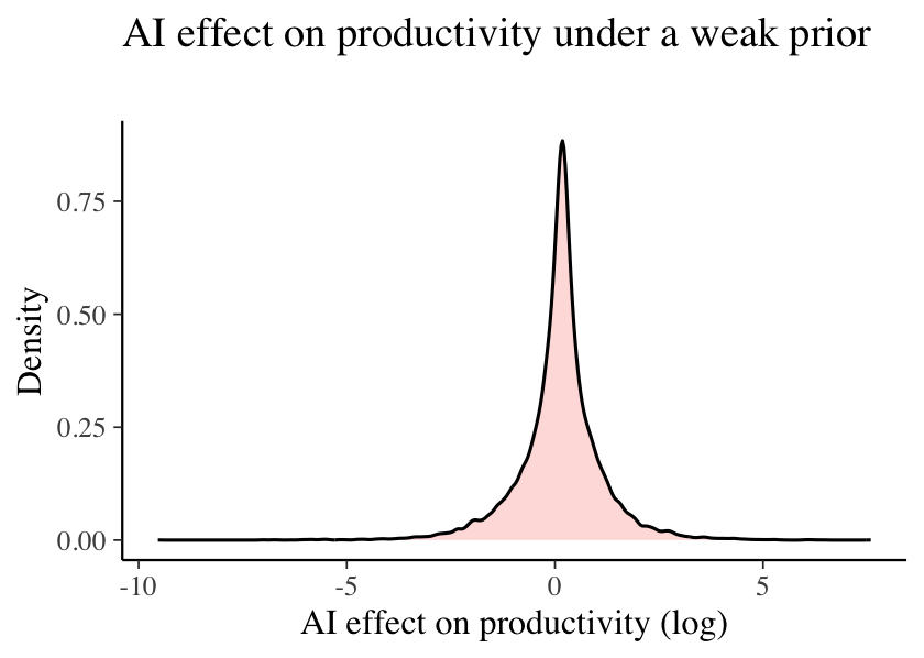
(1) I find some evidence of a AI slowdown under a weak prior. The effect of AI assistance is heavy-tailed. The estimate of shrinks little, by 1-2 percentage points, but the probability of being greater than 0 (slowdown) is only 67% or an odds of 2. We would thereby expect to see effects on the scale of ~8x slower to 8x faster.

Raw info under the box

Aggregate treatment effect (on mean), 1 groups, log-scale:

Hypermean () = 0.12 with 95% interval -1.08 to 1.24

Hyper-SD () = 0.668 with 95% interval 0.027 to 2.013

Posterior predictive effect = 0.12 with 95% interval -2.15 to 2.25

Study-specific effect , log-scale:

mean sd 2.5% 50% 97.5% pooling

0.174 0.080 0.019 0.174 0.329 0.112

External RCT information supports this conclusion

(2-5) Empirical information from RCTs leads to similar results. The modal effects are very similar regardless of prior choice, with the probability of being greater than 0 (slowdown) ranging from 71% to 79%, or an odds of ~3. Similarly, the estimate of remains about 1-2pp smaller than the naive estimator.

The main benefit of empirical priors is to reduce the heaviness of the tails, stabilising the result into a more reasonable ratio. The empirical priors reduces the standard deviation of effects by ~50%, and an additional (multiplicative) ~25% with the hyperprior on . The credible interval of effects ranges from 4.4x slower to 3x faster. This was reduced to 2.8x slower and 2.4x faster when the hyperprior on was included.

Raw info under the box:

Mean treatment effects (), log-scale:

2.5% mean 97.5% median sd

Normal prior -1.081160 0.124269 1.244160 0.151857 0.535624

Askarov without mu -0.814015 0.160512 1.074970 0.168212 0.440329

Askarov with mu -0.408877 0.112773 0.597838 0.123482 0.246115

Cochrane without mu -0.459449 0.164630 0.840410 0.164092 0.303381

Cochrane with mu -0.340188 0.123946 0.528074 0.134874 0.206972

SD for treatment effects (), log-scale:

2.5% mean 97.5% median sd

Normal prior 0.0265147 0.668033 2.012570 0.542467 0.534169

Askarov without mu 0.0740440 0.390271 1.237450 0.303145 0.309621

Askarov with mu 0.0665519 0.319221 0.883557 0.263573 0.218115

Cochrane without mu 0.0413273 0.289254 0.998998 0.214993 0.245435

Cochrane with mu 0.0399904 0.246207 0.766095 0.190886 0.193650

Posterior predictive effects, log-scale:

2.5% mean 97.5% median sd

Normal prior -2.066140 0.126371 2.265210 0.155890 1.000670

Askarov without mu -1.240300 0.161798 1.506120 0.169681 0.655201

Askarov with mu -0.866741 0.114354 1.034730 0.126705 0.452208

Cochrane without mu -0.860214 0.169201 1.194750 0.168411 0.488071

Cochrane with mu -0.696519 0.126310 0.885847 0.142079 0.379580

Study-specific effects (), log-scale:

2.5% median 97.5% mean sd

Normal prior 0.01917045 0.1736704 0.3293063 0.1741994 0.0797464

Askarov without mu 0.01723793 0.173947 0.3294741 0.1737067 0.0796484

Askarov with mu 0.01624105 0.1692157 0.3207828 0.1696944 0.07776433

Cochrane without mu 0.01895238 0.1738501 0.3316292 0.1741977 0.07990579

Cochrane with mu 0.01615038 0.1690724 0.3190106 0.1691452 0.07721711

Posterior probability that mean population effect > 0 (slowdown)

Normal prior 0.66055

Askarov without mu 0.72195

Askarov with mu 0.7187

Cochrane without mu 0.7898

Cochrane with mu 0.77095

Concluding Remarks

Disagreements can be genuine effect differences

The METR uplift study does not provide strong evidence in the direction of the effect or the magnitude of it. We saw that variance in effect sizes differed between the Cochrane and Askarov databases by 50%. I suspect therefore that these estimates are too narrow because the possible effect size of AI interventions is significantly higher as you move from mainly complementary tasks to completely substitutional tasks. This may also explain somewhat the very different predictions elicited from experts versus the recorded result.

Careful metascientific analysis can help

The inability of single studies to correctly identify true average population effects has already been pointed out. We should use metascientific techniques to improve our ability to forecast into the future and provide a stronger evidence basis. In particular, careful construction of prior distributions can reduce the variance in estimates and reveal hidden inappropriate assumptions in our thinking. Model selection remains a difficult problem in strategic forecasting and there is real potential in applying "reference-class borrowing" on a firmer statistical footing.

Acknowledgements

I have adapted the code and information from Zwet, Wiecek and Gelman (2025) under the CC-BY license. Many thanks for a great paper! I also thank the creators and maintainers of BEAR for access to data, as well as the Cochrane review and the Askarov et al. (2023) paper for the provenance of the data.

1. I'll overview the method here, but this method and code is adapted from Zwet, Wiecek and Gelman (2025).
2. Obviously we can't control for the appearance of stronger AI, but we should analyse this from the strength of AI in July 2025.
3. strictly: less bias, better calibration