My Neel Nanda MATS 10.0 Application: Studying Feature Splitting in SAEs via Training Data Attribution

Neel Nanda's MATS 12.0 Applications are open, apply here! I thought I'd share my successful application from December 2025, it includes the executive summary, main content and the logbook I kept throughout!

Here is the original doc I submitted.

Some broad learnings:

• I really overcomplicated this application! Taking gradients through SAEs and doing data attribution was far too complicated and I wish I'd focused on a simpler project with a clearer theory of change and clearer understanding of what a successful project would look like.
• I'm glad I kept a logbook, that really helped with the writeup.
• I wish I'd done best-of-N e.g. spend 2 hours de-risking 4 projects, and choose the one to continue that showed the best signs of life!
• Choosing a project following on from recent Neel MATS projects (check his reposts) is high signal for impactful research areas.
• I didn't leave enough time for the writeup, also doing something so mathsy meant installing a Latex extension in Google Docs and just added a lot of faff!

Executive Summary

Code

SAE latents are not stable across SAE scale or training runs demonstrating feature (or “latent”) splitting. We expand the definition of feature splitting to include SAE latents that split across different training runs. In this project we explore which training documents drive this splitting outcome.

We introduce the first training data attribution study of SAEs by applying influence functions to trace both individual latents and pairs of related latents back to infer the training documents that shaped them. On Gemma-2-2B using Gemma Scope JumpReLU SAEs (layer 3, width 16k, mean ) trained on Pile documents, we run three experiments.

Key Takeaways:

• Feature splitting may be shaped by training data. Data attribution experiments show evidence to support the claim that whether SAE features split or merge is driven by specific documents.
• Influence functions work for SAEs. Adapting influence functions to SAE encoders and decoders is feasible and yields sensible results, while highlighting a key finding: influential examples are related to but not identical to max-activating ones.
• Latent-pair analysis reveals splitting dynamics. In small case studies, we see that documents that push latents together induce coactivation on the same tokens, while documents that pull them apart activate the latents on different tokens.

Experiment 1: Finding the most similar latents

We begin by identifying latents that are "similar" in 3 metrics we define: (1) decoder cosine similarity, (2) activation correlation, and (3) cofiring rate. They serve as good candidates for exploring influential documents on feature splitting.

Experiment 2: Finding an SAE latent’s most influential training docs

We then turn our attention to finding the most influential SAE training documents on the formation of single SAE latent. Given a training document with loss , the influence of on latent is approximated as

where is a damped Gauss-Newton Hessian approximated using EK-FAC, and gradients are taken through the SAE encoder. For a given latent , we define the measurement

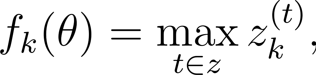
as the maximum activation of latent across token positions in a document.

This “leakage” of the max activating examples into the scoring function is one of the biggest limitations of this method and is addressed in Experiment 3!

I made a Streamlit app to explore the most influential examples and max activating examples:

We report Jaccard@200 of 0.468 ± 0.190 on 20 latents! There are also some latents where the influential documents are rarely the max activating ones which would be cool to explore more!

Experiment 3: Finding documents which push latents together and pull them apart

We extend influence analysis to latent pairs to understand the training dynamics underlying feature splitting. For each pair , we define the measurement as decoder cosine similarity

and use the SAE reconstruction loss

as the training objective, tracking gradients through the decoder.

We analyze 50 latent pairs. For each pair, we compute influence scores using 1,000 Pile documents and extract the top 100 most positive (``pull latents together'') and most negative (``push latents apart'') documents.

We built a Streamlit to examine push and pull documents for each pair, highlighting tokens by latent activation (red = latent only, blue = latent only, green = both). Manual inspection reveals interpretable patterns for some pairs but not others. For the example below, in the push document, both latents activate on the same tokens (often double hyphens). In the pull document, activations occur on distinct tokens.

Future work could explore this further, all of this was run on a node of 4 GH200s so I was a bit compute bottlenecked!

Main Content

Experiment 1: Identifying Candidate Split/Merge Latent Pairs

The goal of Experiment 1 is to identify pairs of SAE latents that plausibly represent split features: cases where a single semantic feature could be represented by one latent but is instead distributed across two or more latents. We operationalize this by searching for latent pairs whose learned representations are already highly similar and whose activations exhibit correlated behavior across data. We compute three key metrics to find split features/merge candidates and using 1,000 Pile documents, we compute these metrics for all 16,384 latents:

(1) Decoder-direction similarity.

Let

denote the SAE decoder, and let

be the decoder direction for latent . We define decoder cosine similarity as

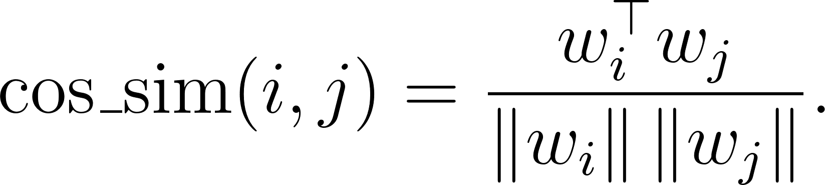
High cosine similarity indicates that the two latents reconstruct activations in similar directions in the model’s activation space, suggesting semantic overlap.

(2) Activation correlation and co-firing.

For each document , let

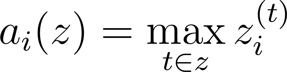
be the maximum activation of latent across token positions. We compute:

• Activation correlation:

measured across a corpus of documents.

• Co-firing rate:

with an analogous definition for

.

(3) Merge score.

We combine these signals into a single merge score:

Latent pairs with high merge scores are strong candidates for feature splitting: they have similar decoder directions and tend to activate together on the same documents.

Results

Using 1,000 Pile documents, we compute these metrics for all 16,384 latents. Figure 1 shows the distribution of latent pairs in decoder similarity vs. activation correlation space and build a Streamlit app to explore latents. We also plot them here for clarity:

Figure 1. Distribution of latent pairs by decoder cosine similarity and activation correlation. Pairs in the upper-right quadrant (high on both metrics) are candidates for split features that could potentially be merged.

Super interestingly, some of these merge candidates appeared to represent different very different concepts from autointerp on neuronpedia but upon closer examination represented the same thing! E.g. 10166 represents repetitions of the letter “t” after an apostrophe and 12675 represents expressions of negative sentiment e.g. “can’t”, “won’t” etc. - totally makes sense that these would be quite similar.

Experiment 2: Training-Data Attribution for Individual Latents

Experiment 2 tests whether influence functions can correctly attribute the formation of individual SAE latents to specific training documents. The hypothesis is that documents with high influence on a latent should often be the ones they fire on or contrasting examples.

I started by plugging SAELens into Kronfluence (a pretty hefty influence function package I’m familiar with) and it was pretty challenging and took longer than I’d’ve liked! A key challenge comes from the JumpReLUSAE module which doesn’t contain any nn.Linear modules for parameters which Kronfluence will track by default. Instead I made a new SAE module which moved W_enc and W_dec into nn.Linear modules without bias so I can track those parameters.

Influence function.

Given a training document with loss , the influence of on latent is approximated as

where is a damped Gauss-Newton Hessian approximated using EK-FAC, and gradients are taken through the SAE encoder.

Measurement.

For a given latent , we define the measurement

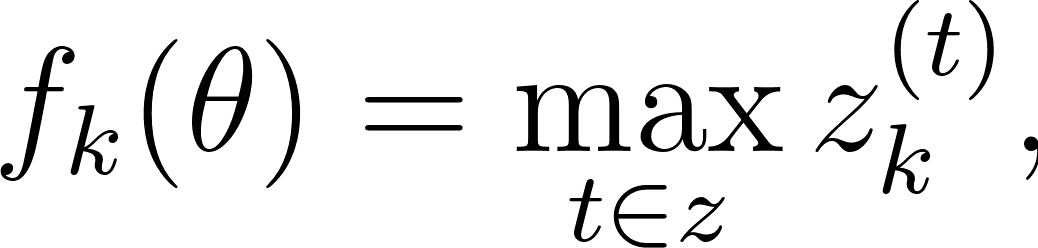
the maximum activation of latent across token positions in a document. This measurement depends on encoder parameters and input activations.

A document with large positive influence increases the maximal activation of latent when upweighted during training, while a document with negative influence suppresses it. If influence functions are meaningful for SAEs, then highly influential documents should overlap substantially with documents where the latent activates most strongly.

For each latent, we compare the top-K most influential documents to the top-K max-activating documents using Jaccard similarity:

where is the set of top-K influential documents and is the set of top-K max-activating documents.

Results

Table 3 shows summary statistics across all 20 latents. The mean Jaccard@200 of 0.468 ± 0.190 indicates substantial overlap - far higher than would be expected by chance (random selection would yield Jaccard ≈ 0.02 for 200 documents from 10,000). This confirms that influence functions at the very least consistently identify semantically relevant training documents.

I think we should be very skeptical though, as I’m using max activating examples to define the query set to calculate the most influential examples - I think this is a limitation of this approach and I have addressed it in Experiment 3!

Another limitation is the size of the dataset. For time’s sake, I have only considered 10k documents from the Pile to calculate Influential and max activating docs. Influence functions can take a lot of time and memory to compute (there are plenty of workarounds and there is at least one paper which calculates influence on billion parameter LLMs on the whole pretraining set using e.g. TFIDF filtering, LoRA gradient approximations) but I don’t have a huge amount of time to do those hehe! Therefore, it would be likely to have good Jaccard with such a small sample size, but with a larger sample size we might see much worse Jaccard. This would be interesting and help us find influential documents which aren’t easy to find via standard max activating approaches.

Experiment 3: Latent-Pair Attribution for Feature Splitting

We extend influence analysis to latent pairs to understand the training dynamics underlying feature splitting. For each pair , we define the measurement as decoder cosine similarity

and use the SAE reconstruction loss as the training objective, tracking gradients through the decoder. Following the standard influence function sign convention, negative influence scores indicate documents that increase the measurement (pushing decoder directions together), while positive scores indicate documents that decrease it (pulling directions apart).

Sampling Strategy. We analyze 50 latent pairs: 25 with the highest merge scores (top candidates for split features) and 25 randomly sampled pairs. The random sample provides a baseline to test whether influence patterns generalize beyond high-similarity pairs. For each pair, we compute influence scores using 1,000 Pile documents and extract the top 100 most positive (``pull'') and most negative (``push'') documents.

Coactivation Analysis. To quantify whether both latents activate together on a document, we define a coactivation score:, where is the activation of latent at token . A score of 1.0 indicates both latents activate equally; 0.0 indicates only one activates.

We define push and pull documents.

Under this sign convention:

• Merging-pressure (push) documents: . Upweighting these documents increases decoder cosine similarity and pushes latents together.
• Splitting-pressure (pull) documents: . Upweighting these documents decreases decoder cosine similarity and pulls latents apart.

Formally, for a fixed K we define

Results

We test the hypothesis

But don’t find evidence that this is the case - interestingly!!

However, some interpretable things I’ve noticed:

Top Merge Candidates

Example 1

For latents 2170 (references to statistical analysis or data metrics) and 7369 (mathematical expressions and operations), the training doc most likely to push the latents together sees both latents activate on the same double hyphen tokens. Whereas the doc most likely to pull latents apart sees latents activate on different tokens.

Example 2

In this example, we see that the push docs often show latent 5287 (puncuation marks and their frequencies) and latent 15297 (terms related to dates, times and temporal sequences) occurring in close proximity whereas the pull docs don’t seem to be very interpretable at all.

Example 3

Often the differences between the push and pull docs aren’t that interpretable (at least to me)

E.g. here the latents 237 (instances of numerical data or statistics) and 5390 (numeric values or references ot dates and events) always seem to fire on 1st and 2nd digit in days consecutively, whether a push document (left) or pull document (right)

Random Candidates

In the random candidates, it’s hard to find any patterns and the documents often have very low latent i and j activations at all. I’m not yet sure why this is, but I might hypothesise that there are much fewer docs where these latents co-appear and therefore few docs are heavily influential.

Log Book

Tags from Neel’s Suggested Research Problems:

• Applied Interpretability -> Other techniques -> Training Data Attribution
• Basic Science -> Basic Science of SAEs
• Novelty -> New ideas

Resources:

• A is for Absorption https://arxiv.org/pdf/2409.14507
  • SAE latents often have lower-than-expected recall
  • Feature splitting - where an SAE latent tracks a general feature in a narrow SAE but splits into multiple more specific SAE latents in a wider SAE
  • Feature absorption - a problematic form of feature splitting where an SAE latent appears to track an interpretable feature, but that latent has seemingly arbitrary exception cases. This could be due to a more specific latent “absorbing” the feature direction and firing in place of the main latent
• https://arxiv.org/abs/2501.16615

Where I want to start:

• Build a tool that finds the most influential SAE training docs for a specific latent
• Study the correlation between an SAE latent firing lots on docs that are deemed “low influence” - maybe something weird is happening there? - could this help understand low recall?
• I also want to look at feature merging and splitting and define a merge metric such that documents of positive influence push features together and documents of negative influence push features apart - maybe there is something to be learned there?

How can I make my life easier:

• Start with a pretrained SAE on a known dataset
• Don’t let the models get too big - although Neel doesn’t care about GPT-2 (jokes) so they need to at least be functional LLMs
• Find code which I can launch off from

Day 1 (Thursday)

2 Hours in

I started by trying to get claude to zero-shot this! Poor claude failed :( so then I went back to try to reproduce some key functions that I would need - in particular finding the max activating examples from the SAE training data (the Pile). This worked well!

6 hours in

On reflection, plugging SAEs into Kronfluence has been pretty hard and took longer than I’d’ve liked! A key challenge comes from the JumpReLUSAE module which doesn’t contain any nn.Linear modules for parameters which Kronfluence will track by default. Instead I made a new module which moved W_enc and W_dec into nn.Linear modules without bias and this seems to have fixed it!

I started by looking at the SAE latent 1085 for “_short” as introduced in A for Absorption. For latent 1085 ("short"), the most influential training documents include Wikipedia articles about "short films", "short stories", cost curves, and other content where "short" appears prominently - demonstrating that influence functions appear to trace SAE features back to their training data origins. I remain skeptical overall as influence functions aren’t an exact science.

Here is Experiment 1 summarized:

# i_is_for_influence

## Summary

This project uses **influence functions** to trace which training documents from the Pile were most influential in forming specific SAE (Sparse Autoencoder) latents.

### Experimental Method

1. **Load models**: Gemma-2-2B via HookedSAETransformer + a pretrained JumpReLU SAE from Gemma-Scope (layer 3, 16k width)

2. **Pre-compute activations**: Extract and cache model activations at the SAE hook point for ~10k Pile training examples

3. **Fit influence factors**: Use Kronfluence (EKFAC strategy) to compute influence factors over the SAE encoder, treating sum-of-squared latent activations as the training loss proxy

4. **Find query examples**: Identify max-activating examples for the target latent (e.g., latent 1085 = "short" concept)

5. **Compute influence scores**: Calculate pairwise influence between each query and all training examples to find which documents most shaped the latent

### Key Result

For latent 1085 ("short"), the most influential training documents include Wikipedia articles about "short films", "short stories", cost curves, and other content where "short" appears prominently—demonstrating that influence functions can trace SAE features back to their training data origins.

See `latent_data_attribution.ipynb` for the full implementation.

What I’m doing next…

So far we’ve got all the plumbing sorted, now it’s time to do some exploration and come up with some good hypotheses to test. I might spend 1-2 hours on this :)

Day 2 (Friday)

7 hours in

Core Question: Why are some SAE latents polysemantic, and can we trace this back to the training data?

Hypothesis: Polysemantic latents arise because semantically distinct concepts frequently co-occur in training documents. TDA should reveal this—if a latent fires on both "legal terms" and "financial terms," the most influential training examples should be documents where these co-occur (contracts, regulatory filings, etc.).

Experimental approach:

• Identify known polysemantic latents (or find them by clustering max-activating examples)
• Run your TDA pipeline on these
• Analyze whether influential training docs contain the co-occurring concepts
• Validation: If you're right, you should be able to predict which concepts will be entangled based on their co-occurrence statistics in the training data

9 hours in

I lost a lot of time in this bit thinking about ways to find polysemantic latents - then realised what I was actually interested in was something completely different! If I’m honest I think the stress just got to me overnight, I really want this project to represent my research aptitude and it’s super disappointing when your work doesn’t reflect that!

Anyways…if I want to look at feature (latent) merging and splitting, I should look for latents with high and low cosine similarity like in the cosine similarity dashboard on neuronpedia:

Couldn’t find any docs on how they did this, but after some thinking and some testing, the values reported here are the decoder cosine similarity - aka whether two latents write in the same direction in residual space. I was able to reproduce those numbers exactly :)

Super interestingly, some of these merge candidates appeared to represent different very different concepts from autointerp on neuronpedia but upon closer examination represented the same thing! E.g. 10166 represents repetitions of the letter “t” after an apostrophe and 12675 represents expressions of negative sentiment e.g. “can’t”, “won’t” etc. - totally makes sense that these would be quite similar.

If I’m honest, I thought I’d see more spuriously correlated latents haha!

11 hours in

Okay so I've got two notebooks, cosine_similarities.ipynb which finds latents that are most promising for being merged and latent_data_attribution.ipynb which finds the most influential SAE training docs on a measurement set. I’m now gonna make a new notebook called merge_latent_data_attribution.ipynb which uses the decoder cosine similarity between two latents I pick in the compute_measurement function to find SAE training docs with the highest influence on this cosine similarity (e.g. i'd imagine negative influence makes them more similar and positive influence pulls them apart).

Day 3 (Monday)

13 hours in

I’ve made this streamlit to explore latent pairs. Each point on the scatter plot represents a pair of latents :)

• The top left of the plots are latents with low decoder cosine similarity but high co-activating rates (e.g. they fire on the same tokens)
• The bottom right are latents that have high decoder cosine similarity but low co-activating rates (e.g. they never fire on the same tokens)
• The top right are latents that have both high decoder cosine similarity and high co-activating rates.

16 hours in

After doing some OOM error fixing and careful memory management I think most of the code is there ready to be run for my experiments. I also spent maybe ~1 hour using Claude Code to help draft the writeup with some experiment plans. I think this will help me make use of the final couple of hours as we’re getting quite close to the deadline!

Learnings: Everything is taking much longer than I expected due to general engineering challenges e.g. making kronfluence compatible with SAELens by rewriting the JumpReLU module, manage OOM errors from caching SAE activations for kronfluence, managing OOM errors for special “compute_measurement” functions that don’t rely on query documents etc! If I subtracted that time I think I’d be 5 hours in - but that’s ambitious research forya!

18 hours in

I built this streamlit to compute the most influential training examples on an SAE vs the max activating examples

There’s often pretty good overlap 🙂

I think we should be very skeptical though, as I’m using max activating examples to define the query set to calculate the most influential examples - I think this is a limitation of this approach and I have addressed it in Experiment 3!

Another limitation is the size of the dataset. For time’s sake, I have only considered 10k documents from the Pile to calculate Influential and max activating docs. Influence functions can take a lot of time and memory to compute (there are plenty of workarounds and there is at least one paper which calculates influence on billion parameter LLMs on the whole pretraining set using e.g. TFIDF filtering, LoRA gradient approximations) but I don’t have a huge amount of time to do those hehe! Therefore, it would be likely to have good Jaccard with such a small sample size, but with a larger sample size we might see much worse Jaccard. This would be interesting and help us find influential documents which aren’t easy to find via standard max activating approaches.

Will resume the final 2 hours after dinner!

20 hours in

I’ve finished the code for experiment 3 so we’re done! I incorporated some writeup time in the previous hours so I will allow myself 1-2 more hours for reviewing the results of a bigger run of experiment 3.

Quite counterintuitively, negative influence scores imply that training document will increase the cosine similarity between latents (push them together) whereas positive influence scores will decrease the cosine similarity between latents (pull them apart).

Some interpretable things I’ve noticed:

Top Merge Candidates

Example 1

For latents 2170 (references to statistical analysis or data metrics) and 7369 (mathematical expressions and operations), the training doc most likely to push the latents together sees both latents activate on the same double hyphen tokens. Whereas the doc most likely to pull latents apart sees latents activate on different tokens.

Example 2

In this example, we see that the push docs often show latent 5287 (puncuation marks and their frequencies) and latent 15297 (terms related to dates, times and temporal sequences) occurring in close proximity whereas the pull docs don’t seem to be very interpretable at all.

Example 3

Often the differences between the push and pull docs aren’t that interpretable (at least to me)

E.g. here the latents 237 (instances of numerical data or statistics) and 5390 (numeric values or references ot dates and events) always seem to fire on 1st and 2nd digit in days consecutively, whether a push document (left) or pull document (right)

Random Candidates

In the random candidates, it’s hard to find any patterns and the documents often have very low latent i and j activations at all. I’m not yet sure why this is, but I might hypothesise that there are much fewer docs where these latents co-appear and therefore few docs are heavily influential.

21.5 hours in

All that’s left to do is some tidying up and copy & pasting from my overleaf :) Will leave that to a less tired J in the morning.