Untie Squared ReLU variant

1 Intro

My collaborator Michael Bukatin came up with an idea: in the hidden projection of MLP, instead of using ReLU, he would duplicate one branch, and initialize two matrices on the two branches separately, and then multiply the two element-wise, then project back as output in the feedforward layer.

As a quick recap, a standard ReLU FFN is:

And we propose adding some complexity before it gets projected back, we can think of it as a modulating field in the hidden space(which is conventionally 4 the model dimension). Rather than a simple ReLU activation, we want to have two ReLU branches and multiply their outputs elementwise:

And he happened to find there has been a similar tweak in this line of research, where Primer documents an optimization through architecture search that a squared ReLU would actually train more efficiently than a plain ReLU, i.e, they use ReLU(xW)² instead of ReLU(xW):

Our variant actually 'unties' the square into two branches of activation:

The untied variant is a more general form of Primer's, given that when Wa = Wb, it would be equivalent to the squared version:

The idea is also a continuation of my collaborator Michael Bukatin's earlier work in multiplicative neural units as a compact way of representing polynomial interactions. He calls it a piecewise bilinear rectifier, g(x,y) = max(0,x)·max(0,y), which is exactly our untied form per neuron. Here we test it in the context of modern transformer FFNs.

2 Experiment setup

Configs

Implementation wise, we use the open-sourced modded-nano-gpt transformer architecture. And inherited the model configs they chose than deliberately choosing it ourselves. We trained on 2*H100.

• 12-layer GPT
• dmodel=768
• 6 attention heads
• FFN hidden dimension: 3,072
• RoPE and QK normalization
• FineWeb-10B
• 49,152 tokens per optimization step
• 1,750 optimization steps
• Muon optimizer

There are two things we want to mention about the variant, per layer the baseline holds 2 × 768 × 3,072 = 4.72M FFN parameters while ours holds 3 × 768 × 3,072 = 7.08M(since we added a whole extra up-projection). So the untied variant got 1.5× the parameters along with 1.5× the compute. If we wanted to match parameters with three matrices, we'd need d_ff = 2,048.

The inheritance also brings in a bias: because the speedrun repo has its learning rate, warmup, optimizer settings and init scale all co-adapted to its own baseline, so the baseline is sitting at a tuned optimum while our variant isn't. We ran no learning-rate sweep for our untied version.

Cosine similarity

Because our focus is partly on the intermediate projection matrices Wa = Wb, we added a proxy cosine similarity to measure the relationship between the two matrices. Cosine similarity defined as:

And we randomly initialized Wa and Wb at the beginning, which means they will be near orthogonal given they are initialized in a high-dimensional space.

Profiling

During training, we used Anthony's profiling repo to isolate the FFN so we can have a breakdown of the FLOPs in transformer block.

3 Results

Loss

After 1750 steps, our variant is almost reaching the same validation loss as the squared baseline, and it took ~18% more wall-clock per step to get there.

Cosine Similarity

During our training, the cosine similarity between Wa and Wb rose quickly from its near-orthogonal initialization and settled around ~0.77.

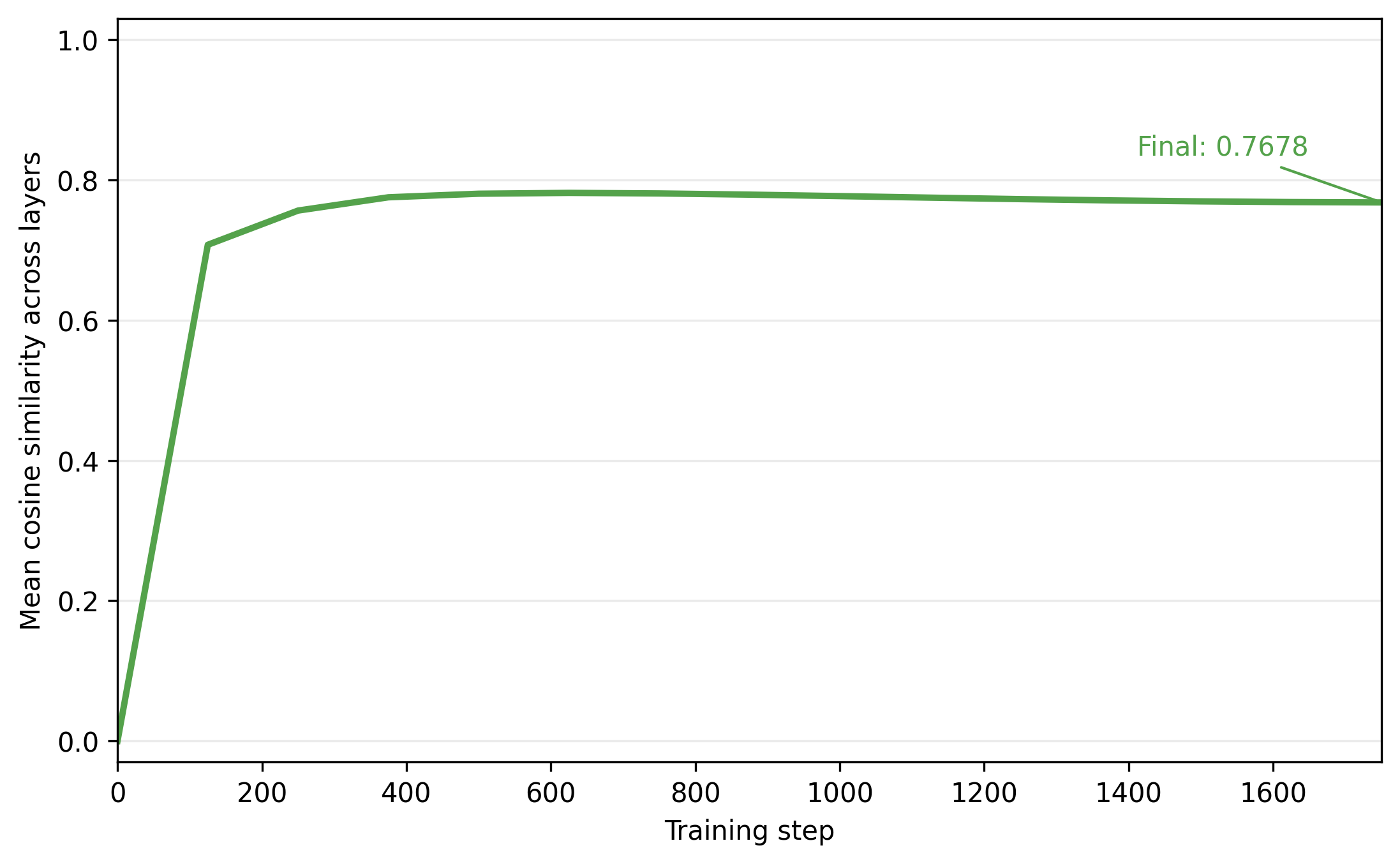
The number was surprisingly high and given it is such a quick convergence, we added a follow-up experiment to initialize with deliberately chosen similarities to see if the pattern breaks or it is a general convergence.

In the follow-up experiment, we initialized Wa and Wb at cosine similarity ≈0 and ≈0.999, tracked both across all 12 layers to step 1,750 (we're using a hidden dimension of 2048 here because it's cheaper than the headline run's 3,072):

After we change the initialization, the pattern breaks. When cosine similarity is initialized at 0.999, during training the two weight matrices actually decreases in cosine similarity. There hence has not been such a universal value the two matrices converge to within our training horizon as we previously suspected.

Measured Flops

The measured FLOPs on 2*H100 is:

Untied variant has a 2.088/1.392 = 1.5 ratio to the Squared ReLU baseline.

4 Some analysis and comparisons

We started the experiment mostly out of curiosity about explainability of transformer, but since we were using modded-nano-gpt(a speedrun repo), and because our variant loses in speed, it shall be time to look into why it slows down the training.

FLOPs analysis

A quick heads-up: FLOPs analysis estimates computational cost: it counts the floating-point additions and multiplications required by the model’s operations.

Preliminaries: Multiplying an matrix by a matrix costs approximately FLOPs. And why? It simply comes from the basic matrix multiplication rule: Multiplying an matrix by a , produces an matrix. Each output entry is the dot product of one row of the first matrix(with shape ) and one column of the second(with shape ). So to produce one output element, it requires k multiplications and k-1 additions. Since there are mn output entries, the total is FLOPs.

With that in mind, we have to look at matrix shapes and how many matrix manipulations we do in the architecture to count the total FLOPs.

A transformer FFN block is a simple up-projection and down-projection. The baseline we chose, squared ReLU, has one up-projection and one down-projection, with an elementwise squared ReLU in between.

Shapes. Before counting, the hidden dimension and the matrices it sizes:

An up-projection expands each token from to dimensions, and the down-projection maps it back to :

In the up-projection, the model is temporarily made “fatter” by design:

this is a common transformer convention dating back to original Transformer, with reason behind that this gives the FFN more hidden features.

Returning to the main point, a standard MLP can be written as:

Very simple, a linear projection, ReLU activation to break linearity, then projected back.

The baseline squared ReLU does this:

with shapes

we can think of the squared ReLU doing a up projection, ReLU activation, then elementwise multiplication(square itself), then down projection. And taking the compute heavy projections into our FLOPs accounting only :

and consider that

The untied variant is two up projections, ReLU activation, then elementwise multiplication, then down projection. Similar to the squared baseline, but we are having an extra up-projection, so three compute heavy matrix multiplications in total :

Using model dimension to express the cost:

Hence, the untied variant’s feedforward projection cost is roughly 3/2=1.5 that of the Squared ReLU baseline.

We can use a computational graph to describe the computation as well. In the forward pass, each projection contributes one matrix multiplication.

During backpropagation(reverse-mode differentiation), we traverse this graph backward. By the chain rule, each projection requires two further matrix multiplications to derive gradients, one with regard to the input and one with regard to the weight, as illustrated in PyTorch's autograd engine. So it will be doubling the number of projection matrix multiplications in the forward pass. The computation ratio between our variant and the baseline is therefore unchanged: 3/2=1.5. And this theoretical analysis actually matches exactly the profiling result 2.088/1.392 = 1.500 as we showed in the Result Section. Though to be fair, the profiler derives GEMM FLOPs from tensor shapes, so this is really a consistency check on our arithmetic.

Wall-Clock time

FLOPs is an algorithmic accounting of the compute, whereas wall-clock is the real-world time. The measured wall-clock time is ~18% slower per step, and there are a few reasons. One is that the FFN takes up only a fraction of the transformer, while attention takes up more compute. A traditional (dense) attention lookup is at complexity of O(n²) while the FFN is at O(n), where n is the sequence length; modded-nanogpt uses sliding-window attention to cut the quadratic term, making it closer to linear, though attention still takes up a large share of the transformer's compute. To put it simply, the FFN slowdown is diluted by the other modules.

Secondly, a modern bottleneck is often not the matrix multiplication itself but HBM bandwidth, like how data is carried between memory and the compute units, something like a CPU stalling on disk writes. It's a traffic jam of data, so a FLOP increase doesn't translate into the same amount of real-world time.

Comparisons

There has been many related architectural designs in the ReLU family. It would make more sense to cross look at the existing ReLU variants. GLUs use one branch to gate the other, for example, ReGLU computes . Squared ReLU is algebraically equivalent to a ReGLU with tied weights(U=V=W), because .

Existing work largely introduce empirical improvements without providing causal explanation for why they work better. Shazeer attributes the success of GLU variants to “divine benevolence.” And just as Anthropic mentioned in their interpretability research, the MLP is hard to explain even for a single layer with a handful of neurons. The model has way more features it wants to represent than it has neurons, so each neuron ends up having polysemanticity, making MLPs difficult to interpret.

And unlike a GLU, our architecture duplicates one branch in the hidden layers of FFN. I think of its symmetric shape as closer to a bilinear layer, though the bilinear design removes the ReLUs and focuses more on interpretability than performance.

5 Conclusion

We replaced a transformer FFN's relu(xW)² with an element-wise product, tested on a 124M modded-nanogpt: FFN projection compute rose 1.5× with no gain in validation loss. The cosine similarity between the two matrices reached ~0.77 under random initialization but didn't converge under a different initialization, so we don't treat the convergence as intrinsic to the architecture. My collaborator also notes the implementation isn't GPU-friendly out of the box. This could be an implementation-hardware mismatch rather than a compute-level failure, leaving room for future kernel-level work.

References

So, D. R., Mańke, W., Liu, H., Dai, Z., Shazeer, N., & Le, Q. V. (2021). Primer: Searching for Efficient Transformers for Language Modeling. arXiv:2109.08668.

Shazeer, N. (2020). GLU Variants Improve Transformer. arXiv:2002.05202.

Elhage, N., et al. (2022). Toy Models of Superposition. Transformer Circuits / arXiv:2209.10652.

Bukatin, M., Matthews, S., & Radul, A. (2016). Dataflow Matrix Machines as Programmable, Dynamically Expandable, Self-Referential Generalized Recurrent Neural Networks. arXiv:1605.05296.

Bukatin, M., & Matthews, S. (2016). Programming Patterns in Dataflow Matrix Machines and Generalized Recurrent Neural Nets. arXiv:1606.09470. (§1.3.2, the piecewise bilinear rectifier g(x,y) = max(0,x)·max(0,y).)

Code and reproducibility. Our fork is at modded-nanogpt-relu-mult, adapted from modded-nanoGPT. Quentin Anthony's profiling repo (torch-profiling-tutorial) was used to isolate the FFN and perform GPU-side FLOP accounting. LLMs (Claude and GPT) were used for coding.

Discuss