Anthropic's J-Lens: A Research Engineer's Analysis

Epistemic status: this is research engineering, not mechanistic interpretability. The compute/cost claims are measured or derived from architecture constants. The quality claims (faithfulness comparisons, spectral channel interpretations) are from one small base model (gpt2-medium), one metric, and in places small samples (n=32); I make no claims about whether the J-space constitutes reasoning or a workspace and this post is about determining what it costs to run the tool in production environments, not the tool's outputs.

All notebooks available here: github.com/willkn/jlens_re

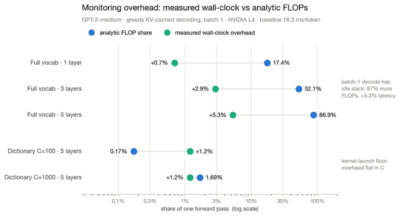
Headline Result: Lens Monitoring is nearly free at decode time with small dictionary size

Anthropic recently released a paper on the transformer circuits platform called ‘Verbalizable Representations Form a Global Workspace in Language Models’. This paper posits that models have an internal workspace where non-verbalised concepts, perhaps certain reasoning steps or other intermediary computations, exist. Anthropic call this the J-Space:

Looking inside the J-Space (Gurnee, W., et al, 2026)

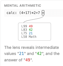
Here is an example from the paper — we see that the model holds certain values in the J-Space when computing an output. One of the core discussions ongoing around this paper is whether the values we observe in the J-Space are useful and if they constitute reasoning. We will not engage with that discussion in this post. Although, I feel that these values have a lot of potential and imagine many practitioners will be looking to implement the techniques into their own experiments or production systems, so this writeup serves as a first venture into analysis of production-level engineering with the J-Space.

Throughout the writeup we will focus our analysis on memory, compute and inference speeds.

The J-Space — an overview

Before we dive into the mathematics, at a high level, how do we access the J-Space? The residual stream is used to determine an output in the final layer by providing a set of logits over a vocabulary, such as the English language. This however is not possible within middle layers as they do not share the same understanding of the residual stream as the final layer does. The paper therefore aims to understand these layers as we do the final layer. To do this, we create an object, the Jacobian, that measures how much the final layer changes (and in which direction) based on some change at an earlier layer. For example, we may observe that an earlier layer is making it more likely that the output will be related to a certain concept.

The formal mathematical definition of the J-Space gives us instant intuition on whether the techniques used are feasible for production environments. To access the J-Space we need to firstly compute a Jacobian, and secondly, apply it at inference time.

Part 1: Computing the Jacobian

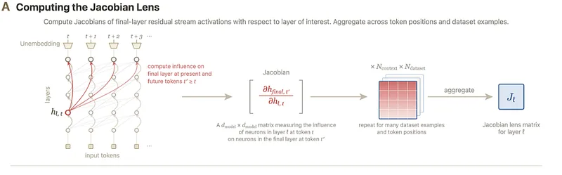
Computing the Jacobian (Gurnee, W., et al, 2026)

Let h_l[t] be the residual stream vector of dimension d at layer l, position t Everything downstream of this vector is a function mapping h_l[t] to the final layer residuals at h_k[t’], where t’ ≥ t since we are using a causal mask (earlier positions can’t attend to later positions to stop the model ‘cheating’).

We then define our Jacobian. For one prompt and one position pair, we run the prompt through the transformer blocks (which can be thought of as a non-linear function f) which produces a final output h_k[t’]:

1.1 h_L[t’] = f(h_l[t])

We can represent this nonlinear function as a Jacobian (which is linear), a collection of these outputs:

1.2 A_l = ∂h_L[t’] / ∂h_l[t]

Every entry in this Jacobian, for example A[i, j], tells us how much coordinate i of the final output vector at position t’ were to shift if we made a small change in the residual stream at layer l. Practically, this encodes the intermediate computations that happen in a forward pass and lets us know what exactly each token changes about the output.

It is helpful to think of intermediate layers in terms of the final layer. In the final layer, we output a word based on the value of the residual vector. In intermediate layers, we have no such thing, and the value of a residual vector in layer 5 might not mean the same thing it does in the final layer. The Jacobian we have here allows us to link non-final layers to the final layers and extract meaning that otherwise would not be found — analogous to a linear map (lossy, non-reversible). However, computing the Jacobian with one prompt gives us a biased view due to taking on individual ‘characteristics’ of that prompt, so we must compute with multiple (n=1000 in the Anthropic paper) to get a better representation:

1.3 A ₗ = (1/N) Σᵢ Aᵢ

This is the general definition of how to obtain a Jacobian for the J-lens. Let's go into some of the engineering tricks Anthropic used to compute theirs in the paper.

The Engineering of Computing a Jacobian

We will first look at how Anthropic determine the Jacobian in the paper.

We call backprop once per output coordinate: inject a one-hot gradient at coordinate i of the final-layer residual (at every valid target position at once) and backpropagate to layer l; each backward returns row i. We then stack these rows to create our final Jacobian. Since backprop passes through every intermediary layer l’ where l’ > l, we can pick up those too and build Jacobians per layer without having to rerun independently. We also need to remember to take averages when computing to destroy the noise that is accumulated by individual prompts or tokens.

In one sentence:

‘ Run backprop once per output coordinate to harvest the Jacobian row by row, with positions averaged inside each pass and prompts averaged across passes — d backwards per prompt, and the average of it all is the J-lens matrix’

Compute required for a Jacobian

Setup

GPT-2-medium (355M, d=1024, L=24, V=50,257), fp32, HF transformers, NVIDIA L4.

Fitting: 128-token WikiText-2 prompts; dim_batch=8 (output dimensions per backward, prompt replicated along the batch axis); first 16 positions excluded (attention sinks); fp32 accumulation; timings synchronised, warm-up passes discarded.

Inference: greedy KV-cached decode, batch 1, 200 new tokens, best of 3; monitor = precomputed W_U x J_L applied in a forward hook. Estimator verified against torch.autograd.functional.jacobian to <10⁻⁶ on a toy model.

Compute/Quality tradeoff

Fitting Cost: The Jacobian requires d_model backward passes per prompt (one vector-Jacobian product per output dimension/coordinate, all layers computed in one backward). Measured on gpt2-medium ( d_model =1024, 355M parameters) on an L4 GPU the observed fitting time followed a cost model of:

2.1 C = 2· N · T · d_model · n_prompts

(where N ≈ 0.95 is an empirically fitted overhead constant and T is sequence length)

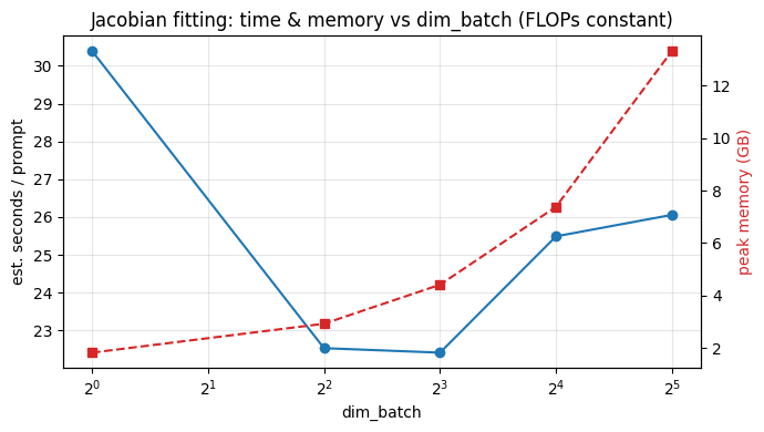
to 5% accuracy, with noise due to overhead. We observed a backward:forward FLOP ratio of 0.95 (we don’t compute parameter gradients since we aren’t updating weights, hence we don’t see the typical 2:1 ratio) but a wall clock ratio of 1.30 (backwards kernels are less efficient). We identified the optimal dim_batch of 8, fitting costs 22.4 s/prompt at 12% MFU, i.e. 8.2×10¹⁶ FLOPs / ~6.7 h for the paper's 1000-prompt recipe

Jacobian fitting: time & memory vs batch size

Fitting with checkpoints allows us to test the quality/cost tradeoff in one run. We used wikitext-2 as our corpus and saw that convergence followed a 1/√n samples law and also beat cross-half floor noise at n=100 prompts, concurring with Anthropic’s claim that 100 prompts is the saturation point for determining a Jacobian. Cross-half floor noise is defined as such:

2.2

JA​=J*+EA​,

JB=J*+EB

JA​−JB​=EA​−EB​

Where Jᵢ is a Jacobian estimated with dataset i and Jⱼ is a dataset j, and there is no overlap between sets Sᵢ ∩ Sⱼ = ∅. This leaves us purely with noise, but of course the complement is the useful component of the Jacobian. This lets us know roughly how similar our Jacobian is to our true optimal…